8 Mixed effects modelling in R-INLA to analysis otolith data
本章では、INLAで線形混合モデルを実行する方法を学ぶ。
8.1 Otoliths in plaice
平衡石(otholith)は魚類の96%にある耳内の器官で、海水から炭化カルシウムを生成して作られている。よって、平衡石の組成を調べればその魚がどこの海域にいたかを推定できる可能性がある。しかし、それを知るためには環境要因と生理的要因がそれぞれどのように平衡石の組成に影響しているかを調べなければならない。
本章では Sturrock et al. (2015) による実験研究のデータを用いる。25個体が7から12ヶ月自然環境に近い状況でタンクに入れて飼育され、生理学的変数(全長、体重、フルトンのcondition factor8、成長率、血漿中のタンパク質、元素濃度)と環境的変数(塩分濃度、温度、海水の元素濃度)が少なくとも1ヶ月ごとに測定された。
\(^7Li, ^{26}Mg, ^{41}K,^{48}Ca, ^{88}Sr, ^{138}Ba\)などの元素濃度が海水中、血漿中、そして平衡石中で測定された。また、性別や魚が生息していた海域、産卵を促すために特定のホルモン(GnRH)を与えられていたかなども測定された。
8.2 Model formulation
Sturrock et al. (2015) では様々な元素濃度を用いたモデリングを行っているが、本章ではそのうちの一つであるSr(ストロンチウム)/Ca(カルシウム)比を応答変数とするモデルの解説を行う。
モデルの共変量としては、性別とGnRHの有無、生息していた海域、環境的変数(塩分濃度、気温、水中のSr濃度、水中のSr/Ca比)と生理学的変数(年齢、全長、体重、condition factor、成長率、血漿中タンパク質、血中Sr濃度、血中Sr/Ca比)が用いられた。交互作用は考えないものとする。
8.3 Dependency
分析するのに十分な平衡石の成長が見られたのは25頭中19頭だけだった。各個体について複数時点のデータがあるため、データは独立ではない(図8.1)。
oto %>%
  mutate(Date = as.Date(Date, format = "%d/%m/%Y")) %>%
  group_by(Fish) %>%
  mutate(date_num = Date - min(Date) + 1) %>%
  ungroup()  -> oto

oto %>%
  ggplot(aes(x = Date, y = O.Sr.Ca))+
  geom_point()+
  scale_x_date(labels = date_format("%m"),
               date_breaks = "2 months") +
  facet_rep_wrap(~Fish, repeat.tick.labels = TRUE)+
  labs(y = "Sr / Ca ratio (mmmol / mol)",
       x = "Time (months)")+
  theme_bw()+
  theme(aspect.ratio = 0.8)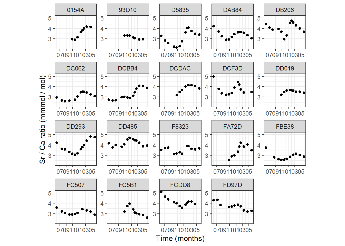
図8.1: Plot of the Sr / Ca ratio versus time for each fish.
ランダム切片に個体IDを入れることでこれについてはある程度対処できる(第4章参照)。この場合、同じ魚からのデータは全て相関\(\phi\)であり、異なる魚の相関は0であると仮定される。ただし、時系列相関は考慮されない。モデル式は大まかに以下のように書ける。本章では分析をシンプルにするため、応答変数が正規分布から得られているとして分析を行う。
\[ \begin{aligned} \rm{Sr/Ca \; ratio} = & \rm{Intercept + Sex + GnRH + Origin} + \\ &+ \rm{lots \; of \; environmental \; variables} \\ &+ \rm{lots \; of \; ephysiological \; variables} \\ &+ \rm{random \; intercept} + noise \end{aligned} \]
8.4 Data exploration
各変数のdotplotを以下に示した(図8.2)。平衡石の成長率(Otolithgrowthrate)のみすこし外れ値があるようだが、他は問題ないようだ。ひとまずはこのまま進む。
oto %>%
  select(Age, Opacity, Growthrate, Otolithgrowthrate,
         B.Sr, B.Sr.Ca, Plasmaprotein,Condition, Totallength,
         O.Sr.Ca, Temp, Sal, SW.Sr, SW.Sr.Ca) %>%
  pivot_longer(everything()) %>%
  group_by(name) %>%
  mutate(n = 1:n()) %>%
  ungroup() %>%
  ggplot(aes(x = value, y = n))+
  geom_point(size = 0.4)+
  facet_rep_wrap(~name, repeat.tick.labels = TRUE,
                 scales = "free")+
  theme_bw()+
  theme(aspect.ratio = 0.8)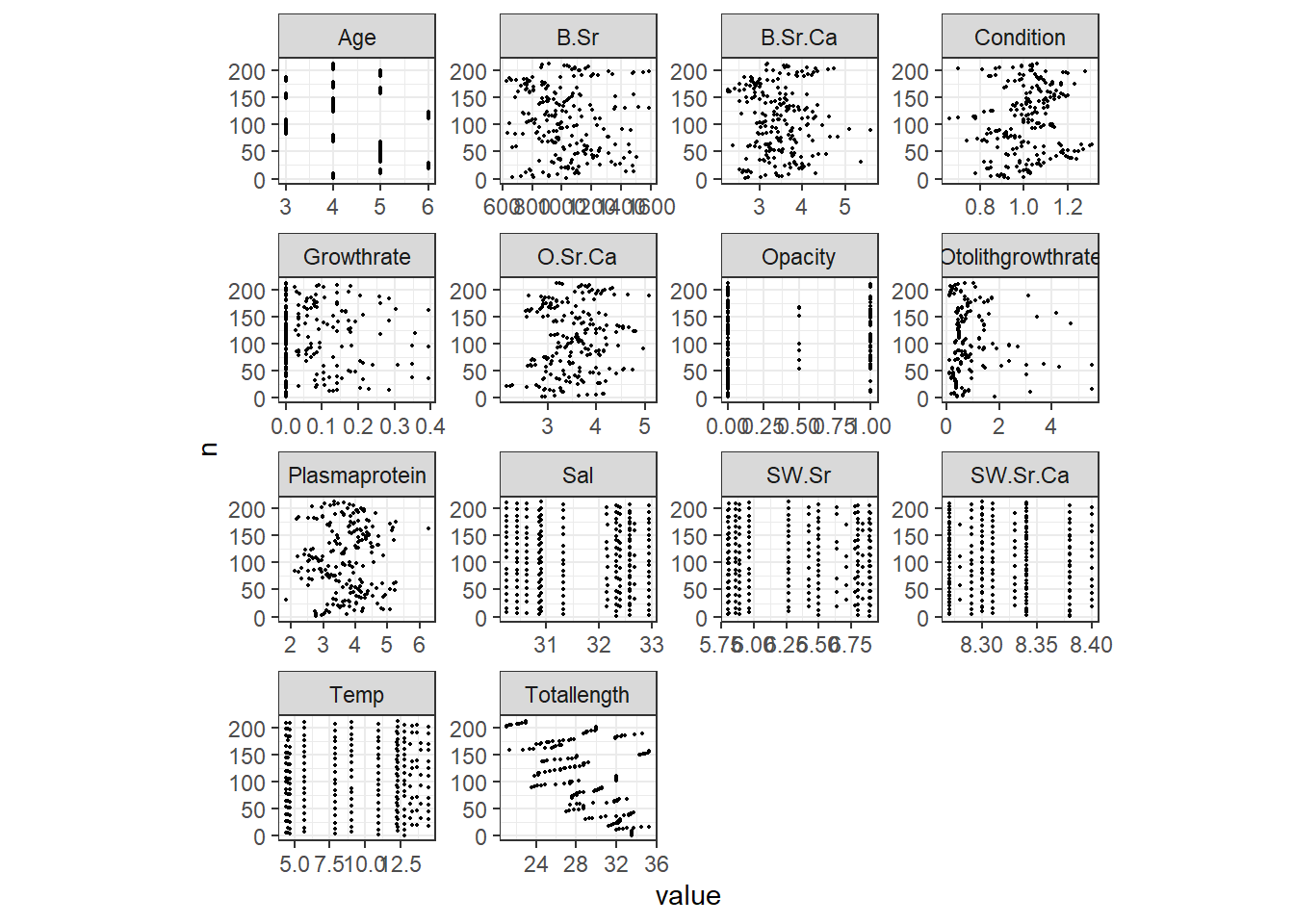
図8.2: Cleveland dotplots of each variable.
現在説明変数がデータ数に対してかなり多い。一般的に、1パラメータ当たり15データが必要だといわれている。そこで、変数の多重共線性を調べて相関の高い変数がないかをVIF(分散拡大係数)で確認する。
library(car)

m9_vif <- lm(O.Sr.Ca ~ Sex + GnRH + Age+ Origin + Opacity + Growthrate+ Otolithgrowthrate +
             B.Sr + B.Sr.Ca + Plasmaprotein + Condition + Totallength+
             Temp + Sal + SW.Sr + SW.Sr.Ca,
             data = oto)

vif(m9_vif) %>%
  data.frame() %>%
  rename(vif=1) %>%
arrange(vif)いくつかVIFの高い変数があることが分かる。ここでは保守的にVIFが3以上の変数は用いないこととする(通常は閾値は5か10で構わない)。海水中のSr濃度(SW.Sr)が最も高いVIF(13.31)を示している。各変数間の相関を調べてみると(図8.3)、気温(Temp)や塩分濃度(Sal)、海中Sr/Ca比(SW.Sr.Ca)と強く相関していることが分かる。よって、これらのどれかを除くとVIFは小さくなりそう。本章では、SW.Srを除くことにする。また、これ以外にVIFが高かった全長(Totallength)も除くことにする。
ggpairs(oto %>%
          select(Age, Opacity, Growthrate, Otolithgrowthrate,
                 B.Sr, B.Sr.Ca, Plasmaprotein,Condition, Totallength,
                 Temp, Sal, SW.Sr, SW.Sr.Ca))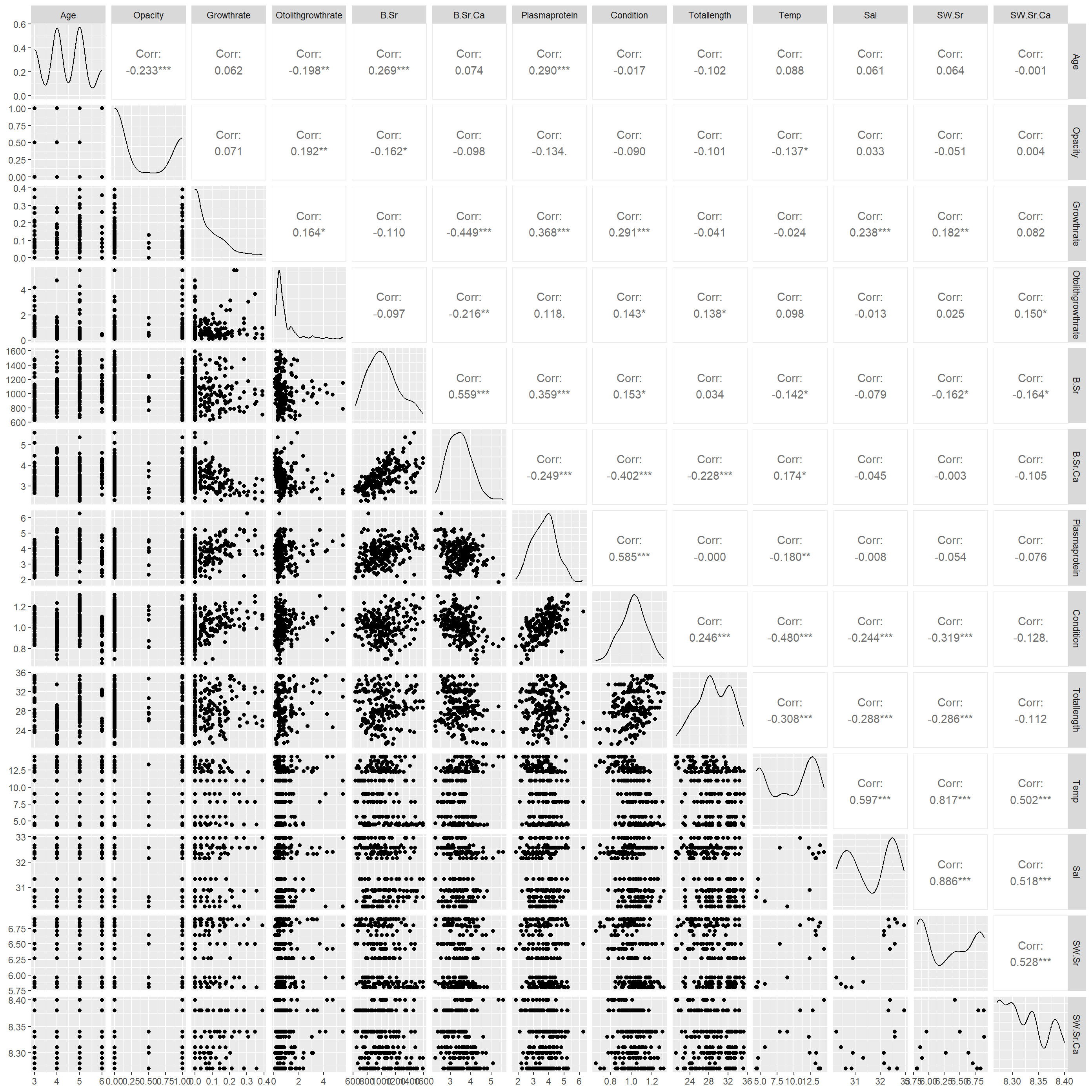
図8.3: Relationship between covariates.
改めてVIFを調べると、まだVIFが3を超えるものが3つだけあることが分かる。血中Sr濃度と血中Sr/Ca比も中程度の相関があるようなので、血中Sr/Ca比を除くことにする。
m9_vif2 <- lm(O.Sr.Ca ~ Sex + GnRH + Age+ Origin + Opacity + Growthrate+ Otolithgrowthrate +
             B.Sr + B.Sr.Ca + Plasmaprotein + Condition + Temp + Sal + SW.Sr.Ca,
             data = oto)

vif(m9_vif2) %>%
  data.frame() %>%
  rename(vif=1) %>%
  arrange(vif)
最終的に全てのVIFが3以下になった。
m9_vif3 <- lm(O.Sr.Ca ~ Sex + GnRH + Age+ Origin + Opacity + Growthrate+ Otolithgrowthrate +
             B.Sr  + Plasmaprotein + Condition + Temp + Sal + SW.Sr.Ca,
             data = oto)

vif(m9_vif3) %>%
  data.frame() %>%
  rename(vif=1) %>%
  arrange(vif)
8.5 Running the model in R-INLA
最終的に選ばれた変数から、以下のようなモデルを実行する。
\[ \begin{aligned} &SrCa_{ij} = \rm{Intercept + Covariates} + a_i + \epsilon_{ij}\\ &a_i \sim N(0, \sigma_{Fish}^2)\\ &\epsilon_{ij} \sim N(0, \sigma^2) \end{aligned} \]
モデルの収束をよくするため、連続値の説明変数は標準化する。Opacityは3つの値(0, 0.5, 1)しか取らないので標準化しなかった。
oto %>%
  select(Fish, O.Sr.Ca, Sex, GnRH, Age, Origin, Growthrate, Otolithgrowthrate,
         B.Sr, Plasmaprotein, Condition, Temp, Sal, SW.Sr.Ca) %>%
  mutate_if(is.numeric, ~scale(.)[,1]) %>%
  mutate(Opacity = oto$Opacity) %>%
  mutate(Date = oto$Date, date_num = oto$date_num) %>%
drop_na() -> oto2モデルは以下の通り。ランダム切片はf(Fish, model = "iid)のように指定する。iidはindependent and identical distributed を表す。すなわち、同じ分布から独立に得られたと仮定するということである。
m9_1 <- inla(O.Sr.Ca ~ Sex + GnRH + Age+ Origin + Opacity + Growthrate+ Otolithgrowthrate +
             B.Sr  + Plasmaprotein + Condition + Temp + Sal + SW.Sr.Ca +
             f(Fish, model = "iid"),
             control.predictor = list(compute = TRUE,
                                      quantiles = c(0.025, 0.975)),
             control.compute = list(dic = TRUE),
data = oto2)固定効果の結果は以下の通り。血中Sr濃度(B.Sr)、血漿中タンパク(Plasmaprotein)、気温(Temp)、塩分濃度Salinityは95%確信区間に0を含んでおらず、これらの変数は影響があるといえそう。
ハイパーパラメータの結果は以下の通り。しかし、前章で見たようにこれらは\(\tau = 1/\sigma^2\)の事後推定値である。
\(\sigma\)と\(\sigma_{Fish}\)の事後平均値は以下のように求められる。
tau <- m9_1$marginals.hyperpar$`Precision for the Gaussian observations`
tau_fish <- m9_1$marginals.hyperpar$`Precision for Fish`

sigma <- inla.emarginal(function(x) 1/sqrt(x), tau)
sigma_fish <- inla.emarginal(function(x) 1/sqrt(x), tau_fish)

c(sigma, sigma_fish)
## [1] 0.6628616 0.4673066級内相関係数は以下の通り。すなわち、同じ個体のデータの相関は0.33くらいであると推定された。
## [1] 0.33199828.6 Model validation
モデルの予測値と残差は以下のように計算できる。
fit9_1 <- m9_1$summary.fitted.values

fit9_1 %>%
  bind_cols(oto2) %>%
  mutate(resid = O.Sr.Ca - mean) -> fit9_1b
残差と予測値にはパターンはなく、等分散性の仮定は満たされていそう。
fit9_1b %>%
  ggplot(aes(x = mean, y = resid))+
  geom_point()+
  theme_bw()+
  theme(aspect.ratio = 1)+
  geom_hline(yintercept = 0,
             linetype = "dashed")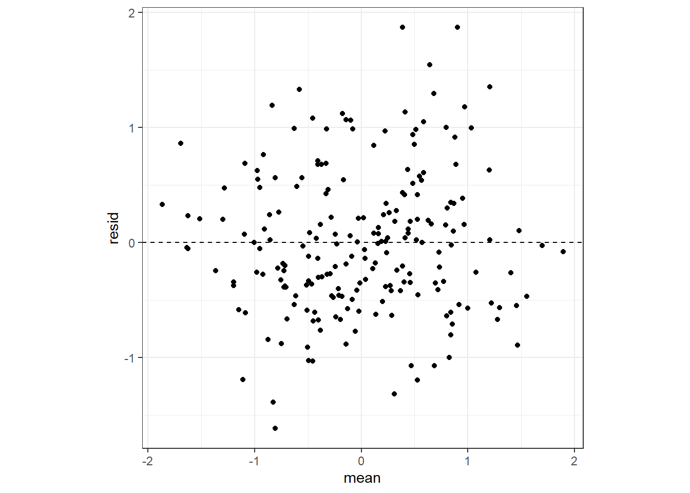
残差と説明変数の関係をプロットしても明確なパターンはなさそう?
fit9_1b %>%
  select(resid, Sex:Opacity) %>%
  select(-Sex, -Origin, -GnRH) %>%
  pivot_longer(2:11) %>%
  ggplot(aes(x = value, y = resid))+
  geom_point(shape = 1)+
  facet_rep_wrap(~name, repeat.tick.labels = TRUE)+
  theme_bw()+
  theme(aspect.ratio = 1)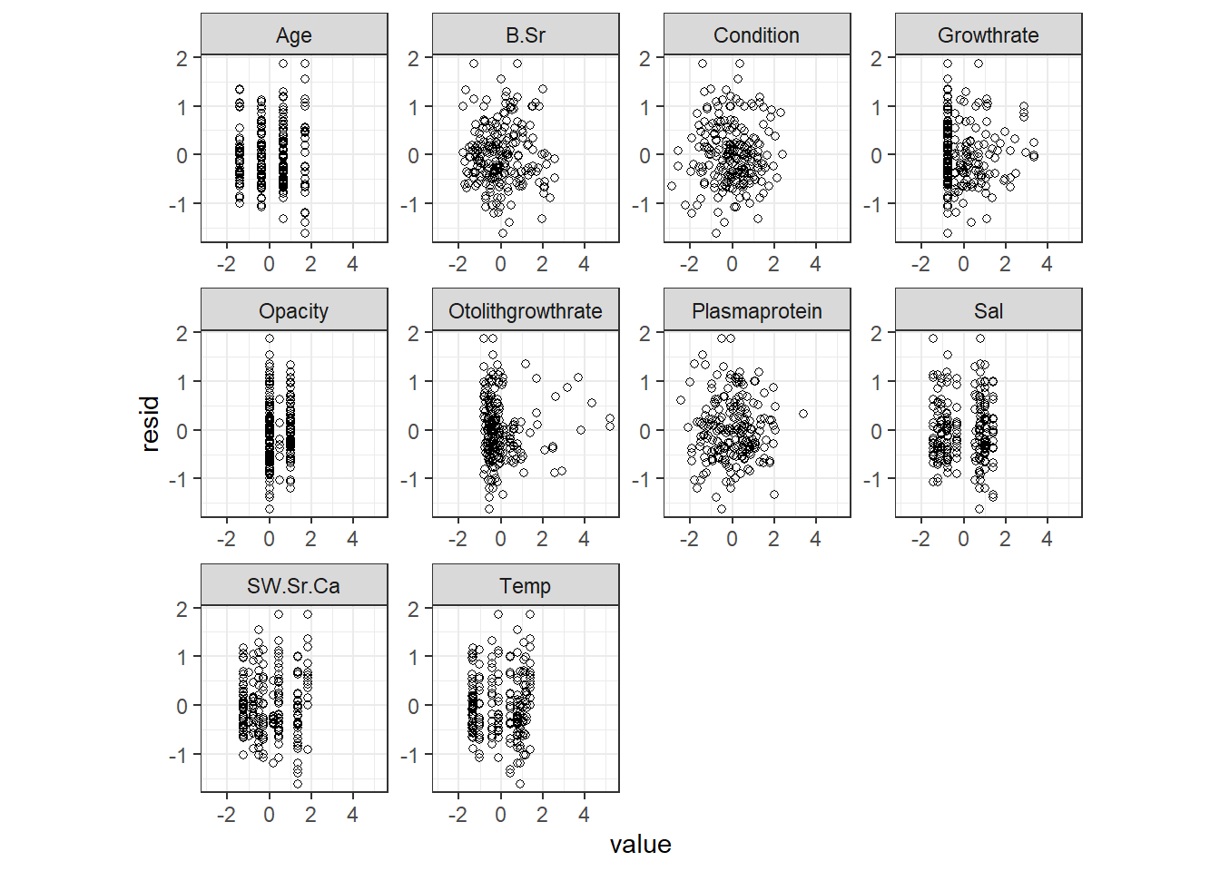
fit9_1b %>%
  select(resid, Sex, Origin, GnRH) %>%
  pivot_longer(2:4) %>%
  ggplot(aes(x = value, y = resid))+
  geom_boxplot(shape = 1)+
  facet_rep_wrap(~name, repeat.tick.labels = TRUE,
                 scales = "free")+
  theme_bw()+
  theme(aspect.ratio = 1)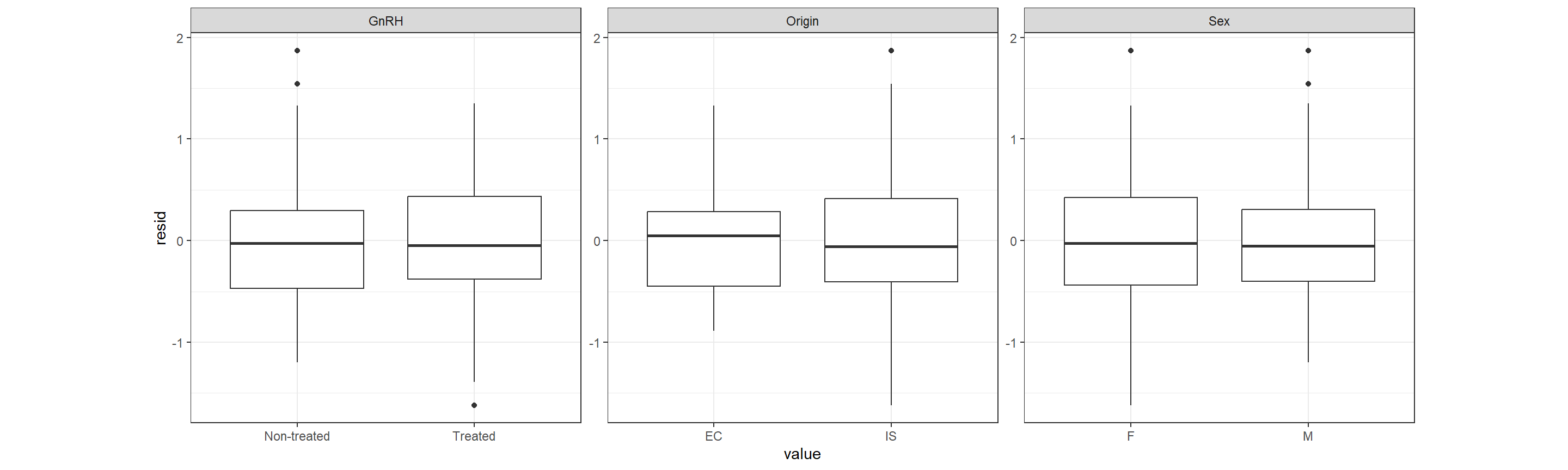
QQプロットを見ても問題はなさそう。残差の正規性も問題ない。
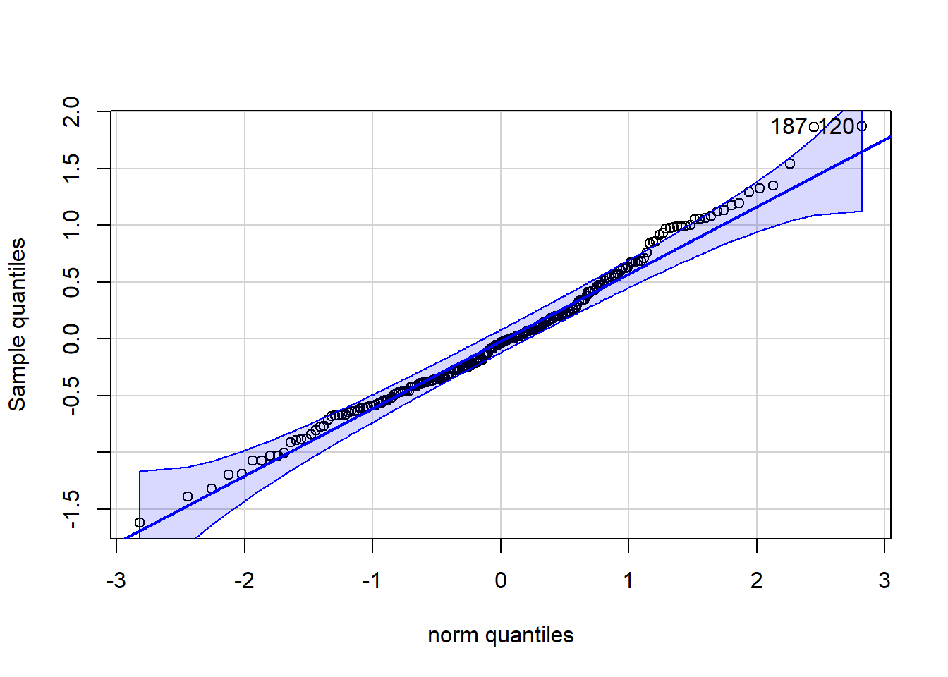
## [1] 120 187最後に、残差の時系列相関があるかを確認する。図を見ると明確に時間的に近いポイントで残差が類似した値をとっていることが見て取れる。すなわち、残差は独立ではなく時系列相関が存在すると考えられる。
fit9_1b %>%
  ggplot(aes(x = Date, y = resid))+
  geom_point(shape = 1)+
  scale_x_date(labels = date_format("%m"),
               date_breaks = "2 months")+
  geom_hline(yintercept = 0)+
  theme_bw()+
  theme(aspect.ratio = 0.8)+
  facet_rep_wrap(~Fish, repeat.tick.labels = TRUE)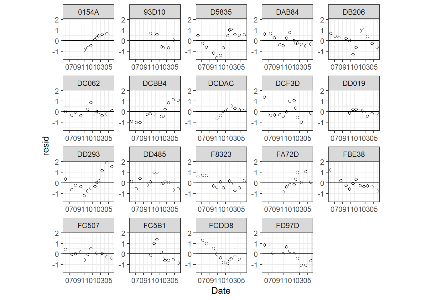
本来はここで時系列相関を考慮したモデルを作るべきだが、ひとまずここではこのまま解説を続ける。続いて、ランダム効果の前提が満たされているかも確認する。
各個体の\(a_i\)の事後分布の要約統計量は以下のように確認できる。
19個しかないのでその正規性をきちんと検討することはできないが、QQプロットを見る限りそこまで大きな問題はなさそう?
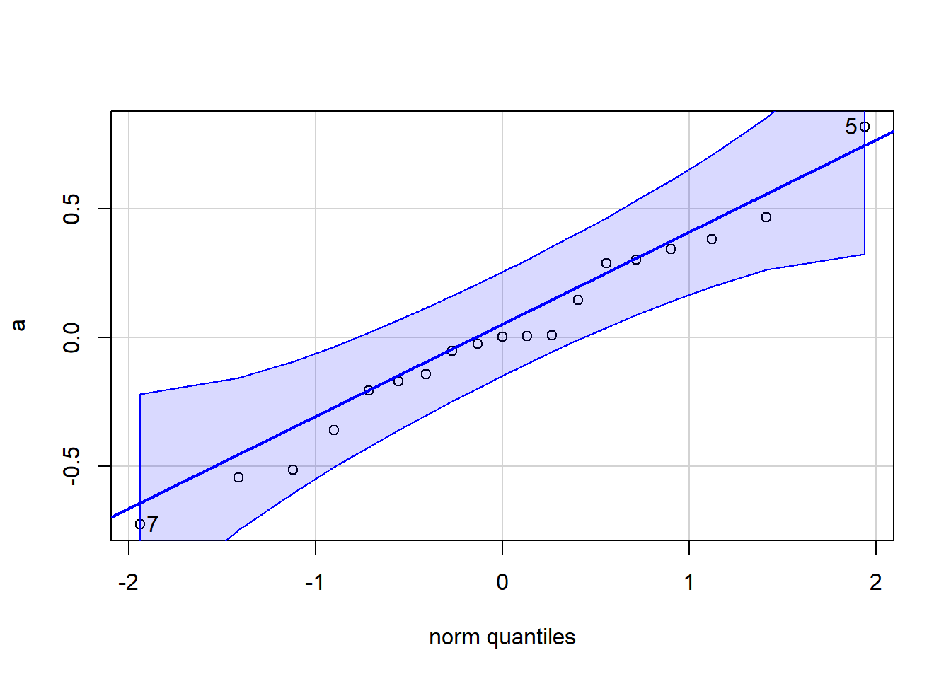
## [1] 5 78.8 Model interpretation
モデルを解釈する際には、結果を可視化することが重要だ。ある説明変数と応答変数の関係についてみる場合には、それ以外の説明変数を固定する必要がある。通常は連続変数であれば平均を(今回は標準化しているので全て0)、離散変数であれば特定の水準に固定することが多い。これを行う方法は2つあるが、そのうち一つは前章(7.6)で解説したので、本節ではもう一つの方法も解説する。
8.8.1 Option 1 for prediction: Adding extra data
まずは前章でも見た一つ目の方法で行う。以下では、血漿中タンパク質とSr/Ca比の関連についてプロットする。ここでは、ランダム効果を含まない予測値を図示したいので、Fish = NAとする。また、連続変数は血漿中タンパク質以外は0(Opacityだけ標準化されていないので平均をとる)、離散変数についてはOrigin‘はEC(English channel)、GnRHはNon-treated、SexはF`に固定する。
newdata <- data.frame(O.Sr.Ca = rep(NA, 25),#
                      Fish = factor(NA, levels =levels(oto2$Fish)),
                      Sex = factor("F", levels = c("F", "M")),
                      Origin = factor("EC", levels = c("EC", "IS")),
                      GnRH = factor("Non-treated", levels = c("Non-treated","Treated")),
                      Temp = 0,
                      Sal = 0,
                      SW.Sr.Ca = 0,
                      B.Sr = 0,
                      Plasmaprotein = seq(from = min(oto2$Plasmaprotein), to =max(oto2$Plasmaprotein), length = 100),
                      Condition = 0,
                      Age = 0,
                      Opacity = mean(oto2$Opacity),
                      Growthrate = 0,
                      Otolithgrowthrate = 0 )

oto3 <- bind_rows(oto2, newdata) %>%
  select(-Date, -date_num)
それでは、実際にモデルを回して予測値と95%確信区間を得る。
m9_2 <- inla(O.Sr.Ca ~ Sex + GnRH + Age+ Origin + Opacity + Growthrate+ Otolithgrowthrate +
             B.Sr  + Plasmaprotein + Condition + Temp + Sal + SW.Sr.Ca +
             f(Fish, model = "iid"),
             control.predictor = list(compute = TRUE,
                                      quantiles = c(0.025, 0.975)),
             control.compute = list(dic = TRUE),
             data = oto3)
以下に結果を図示する。事後平均を用いた平均の予測値と、その95%確信区間である。
fit9_2 <- m9_2$summary.fitted.values[210:309,] %>%
  bind_cols(newdata) %>%
  ## 血漿中タンパク質は元のスケールに戻す
  mutate(Plasmaprotein = Plasmaprotein*sd(oto2$Plasmaprotein) + mean(oto2$Plasmaprotein))

fit9_2 %>%
  ggplot(aes(x = Plasmaprotein))+
  geom_line(aes(y = mean))+
  geom_ribbon(aes(ymin = `0.025quant`, ymax = `0.975quant`),
              alpha = 0.3)+
  geom_point(data = oto2,
             aes(y = O.Sr.Ca),
             shape = 1)+
  theme_bw()+
  theme(aspect.ratio = 1)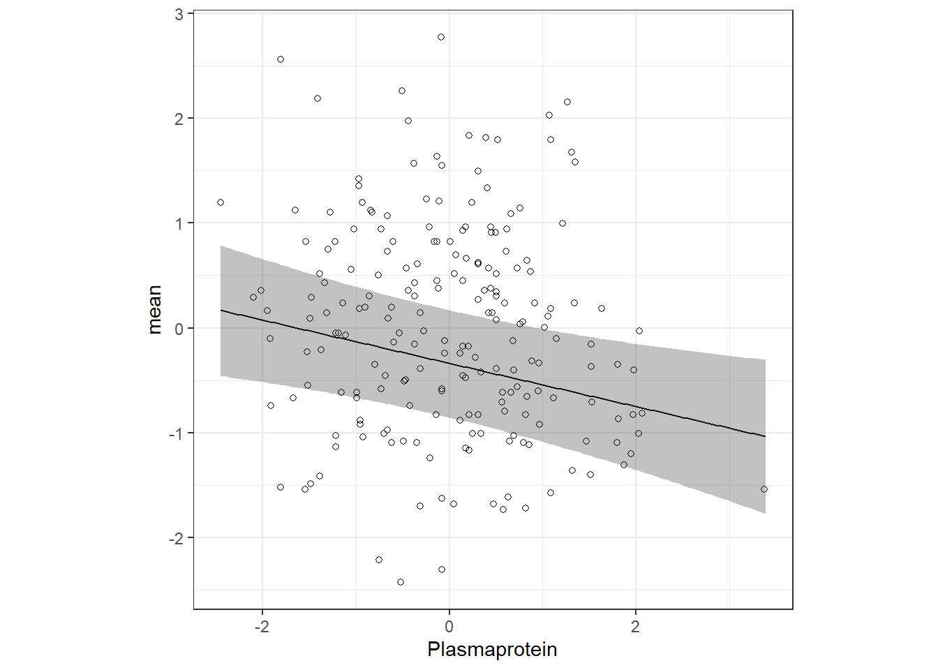
8.8.2 Option 2 for prediction: Using the inla.make.lincombs
続いて、もう一つの方法を解説する。ここでは、inla.make.limcombsを使用する。先ほどと全く同じではないが似た結果が得られる。
まず、1つ目の方法と同様に予測値が欲しい範囲の変数を格納したデータフレームを作る。ただし、このときランダム効果と応答変数は含めなくていい。
newdata2 <- data.frame(Sex = factor("F", levels = c("F", "M")),
                       Origin = factor("EC", levels = c("EC", "IS")),
                       GnRH = factor("Non-treated", levels = c("Non-treated","Treated")),
                       Temp = 0,
                       Sal = 0,
                       SW.Sr.Ca = 0,
                       B.Sr = 0,
                       Plasmaprotein = seq(from = min(oto2$Plasmaprotein), to =max(oto2$Plasmaprotein), length = 100),
                       Condition = 0,
                       Age = 0,
                       Opacity = mean(oto2$Opacity),
                       Growthrate = 0,
                       Otolithgrowthrate = 0 )
次に、これらを切片を含むマトリックスにする。
Xmat <- model.matrix(~ Sex + GnRH + Age+ Origin + Opacity + Growthrate+ Otolithgrowthrate +
                       B.Sr  + Plasmaprotein + Condition + Temp + Sal + SW.Sr.Ca,
                     data = newdata2)
最後にこれをデータフレームにする。
それでは、inlaでモデルを実行する。このとき、あらかじめXmatを変換する必要がある。その後、inlaでlimcomb =(linear combinationの意)で作成したオブジェクトを指定する。
lcb <- inla.make.lincombs(Xmat)

m9_3 <- inla(O.Sr.Ca ~ Sex + GnRH + Age+ Origin + Opacity + Growthrate+ Otolithgrowthrate +
             B.Sr  + Plasmaprotein + Condition + Temp + Sal + SW.Sr.Ca +
             f(Fish, model = "iid"),
             lincomb = lcb,
             family = "gaussian",
             control.predictor = list(compute = TRUE,
                                      quantiles = c(0.025, 0.975)),
data = oto2)m9_3$summary.lincomb.derivedに予測値と確信区間が格納されているので、これをnewdata2と結合する。
fit9_3 <- m9_3$summary.lincomb.derived %>%
  bind_cols(newdata2) %>%
  mutate(Plasmaprotein = Plasmaprotein*sd(oto2$Plasmaprotein) + mean(oto2$Plasmaprotein))
最後にこれを図示する。
fit9_3 %>%
  ggplot(aes(x = Plasmaprotein))+
  geom_line(aes(y = mean))+
  geom_ribbon(aes(ymin = `0.025quant`, ymax = `0.975quant`),
              alpha = 0.3)+
  geom_point(data = oto2,
             aes(y = O.Sr.Ca),
             shape = 1)+
  theme_bw()+
  theme(aspect.ratio = 1)
8.10 Changin prior of fixed parameters
本稿では、ここまで事前分布にINLAのデフォルトを使用してきた。しかし、今回のように1湯のランダム切片しか持たないときは問題ないが、ランダム効果を2つ以上持つ場合や、それらに時空間的相関を仮定するときには、事前分布の影響を確認した方がよい。
INLAでは固定効果のパラメータのデフォルトの事前分布は平均0で精度$\(0.001の正規分布になっている。\)\(を\)\(に直すと、\)= 31.62$である。
\[ \beta_i \sim N(0, 31.6^2) \]
正規分布では\(±3 \times \sigma\)の範囲に99%の値が入るので、この事前分布はパラメータがおよそ-95.8から94.8の値をとることを贈呈していることになる。これは十分に広い。なお、切片のパラメータの精度は0にされている。
以下では、事前分布を変えたときに結果がどのように変化するかを見ていく。話を単純にするため、先ほどの結果で影響があった4つの変数のみをモデルに含める。また、変数変換は行わないものとする。
まず、デフォルトの事前分布でモデリングを行う。
m9_4a <- inla(O.Sr.Ca ~ B.Sr  + Plasmaprotein +  Temp + Sal  +
             f(Fish, model = "iid"),
             family = "gaussian",
             data = oto)
得られたハイパーパラメータ以外の事後分布の要約統計量は以下の通り。
それでは、次に情報事前分布を用いてモデルを回す。ここでは、例えば先行研究などの結果からPlasmaproteinの回帰係数\(\beta_{Plasma}\)が以下の事前分布を持つとする。
\[ \beta_{Plasma} \sim N(-0.22, 0.01^2) \]
\(\sigma = 0.01\)のとき\(\tau = 10000\)である。一方で、その他のパラメータはデフォルトと同様に平均0で精度0.001の無情報事前分布を事前分布に定める。また、切片のパラメータの事前分布もデフォルトと同様である。inlaでは、control.fixedオプションで事前分布を指定できる。
m9_4b <- inla(O.Sr.Ca ~ B.Sr  + Plasmaprotein +  Temp + Sal  + f(Fish, model = "iid"),
              control.fixed = list(mean = list(Plasmaprotein = -0.22, Temp = 0, Sal = 0, B.Sr = 0),
                                   prec = list(Temp = 0.001, Sal = 0.001, B.Sr = 0.001, Plasmaprotein = 10000),
                                   mean.intercept = 0,
                                   prec.intercept = 0),
              data = oto)
血漿中タンパクの回帰係数の推定値がかなり変わっている。
結果が明らかにおかしい。何らかのバグ?おそらく事前分布の平均が反映されていない。
8.11 Changing priors of hyperparameters
先ほどのモデルにはハイパーパラメータが2つあった(\(\sigma\)と\(\sigma_{Fish}\))。しかし、INLAでは精度(\(\tau = 1/\sigma^2, \tau_{Fish} = 1/\sigma_{Fish}^2\)が推定される。これらのデフォルトの事前分布は以下の通り。これは、\(\tau\)と\(\tau_{Fish}\))がガンマ分布を事前分布に持つのと同じことである。
\[ \begin{aligned} &log(\tau) \sim LogGamma(1, 0.00005)\\ &log(\tau_{Fish}) \sim LogGamma(1, 0.00005)\\ \end{aligned} \]
ガンマ分布は2つのパラメータshapeとscaleを持っており、それぞれ\(a\)とと\(b\)で示されることが多い。ただし、INLAでは\(b\)をscaleパラメータの逆数に用いているためややこしい。以下では、INLAと同様にscaleパラメータの逆数(rateパラメータという)を\(b\)で示す。このとき、ガンマ分布の平均は\(a/b\)で分散は\(a/b^2\)となる。
INLAでは、\(\tau\)と\(\tau_{Fish}\)の事前分布に\(Gamma(a = 1, b = 0.00001)\)を設定している。これは、ほぼ一様分布のようになる(図8.4のA)。一方で、 Carroll et al. (2015) は、INLAではポワソンGLMMのときには\(Gamma(1, 0.5)\)の方がデフォルトよりもうまく分析できることを示している。この時のガンマ分布は図8.4のBのようになる。
x <- seq(0, 20, length = 1000)

data.frame(x = x,
           y = dgamma(x, shape =1, rate = 0.00001)) %>%
  ggplot()+
  geom_line(aes(x = x, y = y))+
  coord_cartesian(ylim = c(0,0.00001))+
  theme_bw()+
  theme(aspect.ratio = 1)+
  labs(title = "A: shape =, rate = 0.00001")-> p1

data.frame(x = x,
           y = dgamma(x, shape =1, rate = 0.5)) %>%
  ggplot()+
  geom_line(aes(x = x, y = y))+
  coord_cartesian(ylim = c(0,0.5))+
  theme_bw()+
  theme(aspect.ratio = 1)+
  labs(title = "B: shape = 1, rate = 0.5")-> p2

p1 + p2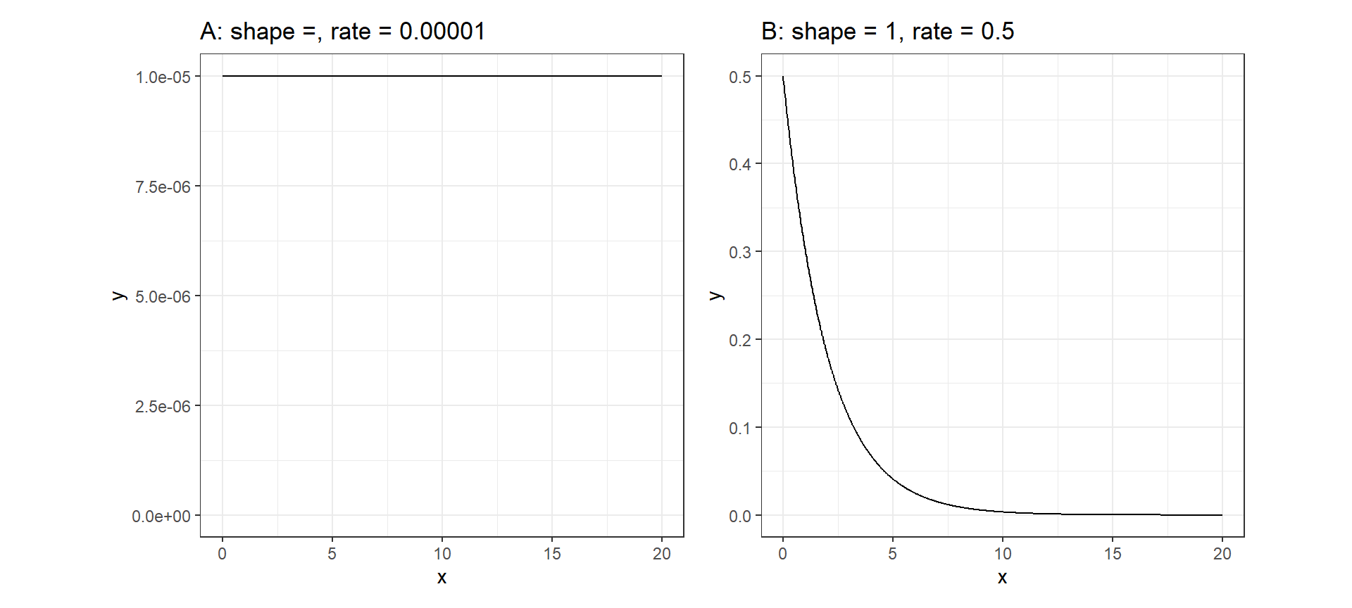
図8.4: Gamma distribution with shape = 1 and rate = 0.00001.
では、\(\tau\)が\(Gamma(1,0.5)\)に従うとき、\(\sigma\)はどのような値をとるだろうか。シミュレーションによってこの分布から\(\tau\)をランダムに抽出したときの\(\sigma\)の値の分布を示したのが図8.5である。ここから、この事前分布では\(\sigma\)はおおよそ0から5までの間の値をとることが多いことが分かる。
set.seed(123)
tau <- rgamma(n = 1000, shape = 1, rate = 0.5)

data.frame(sigma = 1/sqrt(tau)) %>%
  ggplot(aes(x = sigma))+
  geom_histogram(binwidth = 1,
                 alpha = 0,
                 color = "black")+
  theme_bw()+
  theme(aspect.ratio = 1)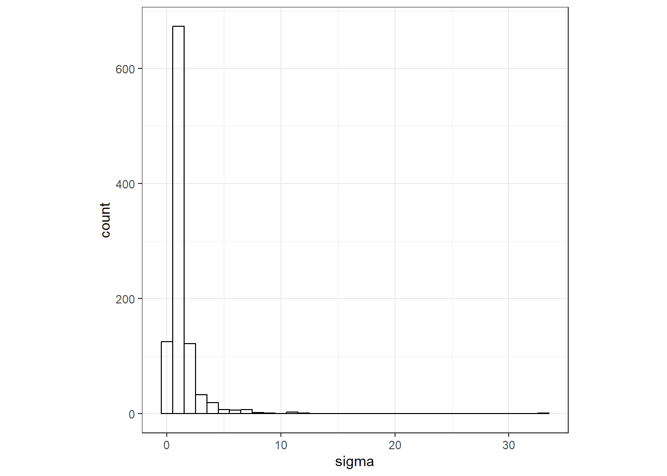
図8.5: 1000 simulated values of sigmas when sampling tau from Gamma(1, 0.5)
ただし、 Carroll et al. (2015) はポワソン分布の場合の話であり、リンク関数にログ関数を用いていることは注意が必要である。私たちが現在使っているのは正規分布のモデルでリンク関数は恒等関数である。
さて、それではハイパーパラメータの事前分布を変えたときに結果がどのように変わるかを見てみる。\(\sigma\)の事前分布はcontrol.familyオプションで、\(\sigma_{Fish}\)の事前分布は式のf(Fish, model = "iid", ...)の中で指定できる。まずは、デフォルト(\(\sigma, \sigma_{Fish} \sim Gamma(1,0.00001)\)のモデルを回す。
続いて、事前分布に\(\sigma, \sigma_{Fish} \sim Gamma(1,0.5)\)を用いてみる。
m9_5b <- inla(O.Sr.Ca ~ B.Sr  + Plasmaprotein +  Temp + Sal  +
                f(Fish, model = "iid",
                  hyper = list(prec = list(prior = "loggamma",
                                           param = c(1,0.5)))),
              control.family = list(hyper = list(prec = list( prior = "loggamma",
                                                              param = c(1, 0.5)))),
              data = oto)
固定効果の推定値や95%確信区間などはほとんど変わらなかった。
m9_5a$summary.fixed %>%
  select(1,2,3,5) %>%
  mutate(model = "m9_5a") %>%
  rownames_to_column(var = "Parameter") %>%
  bind_rows(m9_5b$summary.fixed %>%
  select(1,2,3,5) %>%
  mutate(model = "m9_5b") %>%
rownames_to_column(var = "Parameter"))一方で、推定されたハイパーパラメータの事後分布を示すと、特に\(\sigma_{Fish}\)はかなり違うことが分かる。
tau5a <- m9_5a$marginals.hyperpar$`Precision for the Gaussian observations`
tau5b <- m9_5b$marginals.hyperpar$`Precision for the Gaussian observations`
tau_fish5a <- m9_5a$marginals.hyperpar$`Precision for Fish`
tau_fish5b <- m9_5b$marginals.hyperpar$`Precision for Fish`

## sigmaにする
myfun <- function(x) 1/sqrt(x)

sigma5a <- inla.tmarginal(myfun, tau5a) %>% data.frame() %>% mutate(model = "m9_5a")
sigma5b <- inla.tmarginal(myfun, tau5b) %>% data.frame() %>% mutate(model = "m9_5b")
sigma_fish5a <- inla.tmarginal(myfun, tau_fish5a) %>% data.frame() %>% mutate(model = "m9_5a")
sigma_fish5b <- inla.tmarginal(myfun, tau_fish5b) %>% data.frame() %>% mutate(model = "m9_5b")

## 図示
sigma5a %>%
  bind_rows(sigma5b) %>%
  ggplot(aes(x = x, y = y))+
  geom_line(aes(color = model))+
  scale_color_manual(values = c("red","blue"))+
  theme_bw()+
  theme(aspect.ratio = 1)+
  guides(color = "none")+
  labs(x = expression(sigma),
       y = expression(paste("Pr(", sigma, "|D)"))) -> p1

sigma_fish5a %>%
  bind_rows(sigma_fish5b) %>%
  ggplot(aes(x = x, y = y))+
  geom_line(aes(color = model))+
  scale_color_manual(values = c("red","blue"))+
  theme_bw()+
  theme(aspect.ratio = 1)+
  labs(x = expression(sigma[Fish]),
       y = expression(paste("Pr(", sigma[Fish], "|D)")))-> p2

p1 + p2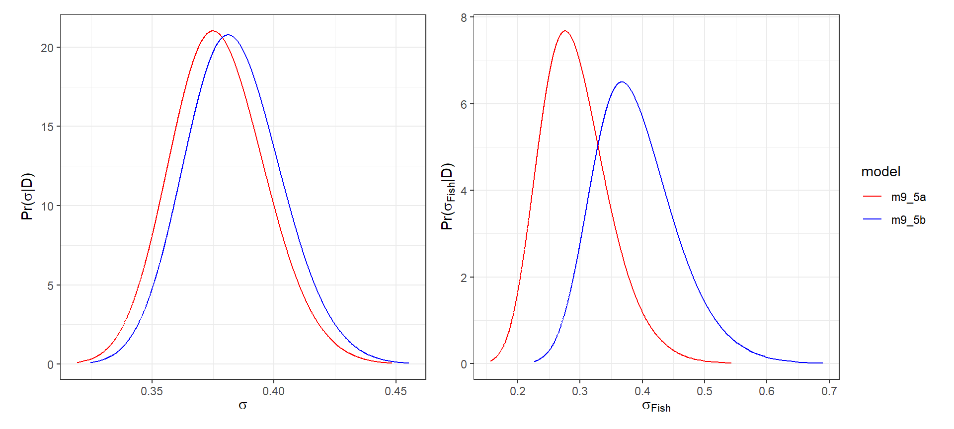
References
体重/体調^3 × 1000で与えられる。↩︎