4 Linear mixed-effects models and dependency
本節では、混合モデルがどのようにデータの非独立性に対処しているのかを見ていく。
4.1 White Storks
ここでは、シュバシコウの成長に影響を与える要因を調べた Bouriach et al. (2015) の研究データを用いる。あるコロニー内の多くの巣から、各巣内の複数の雛のデータが複数回ずつにわたって最大生後54日まで収集されている。
雛の成長度合いは、くちばし長で評価されている。図4.1は年齢とくちばし長の関連を図示したものである。
ws %>%
  ggplot(aes(x = age, y = beak))+
  geom_point(shape =1,
             size = 1.5)+
  theme_bw()+
  theme(aspect.ratio = 1)+
  labs(y = "Beak length",
       x = "Age")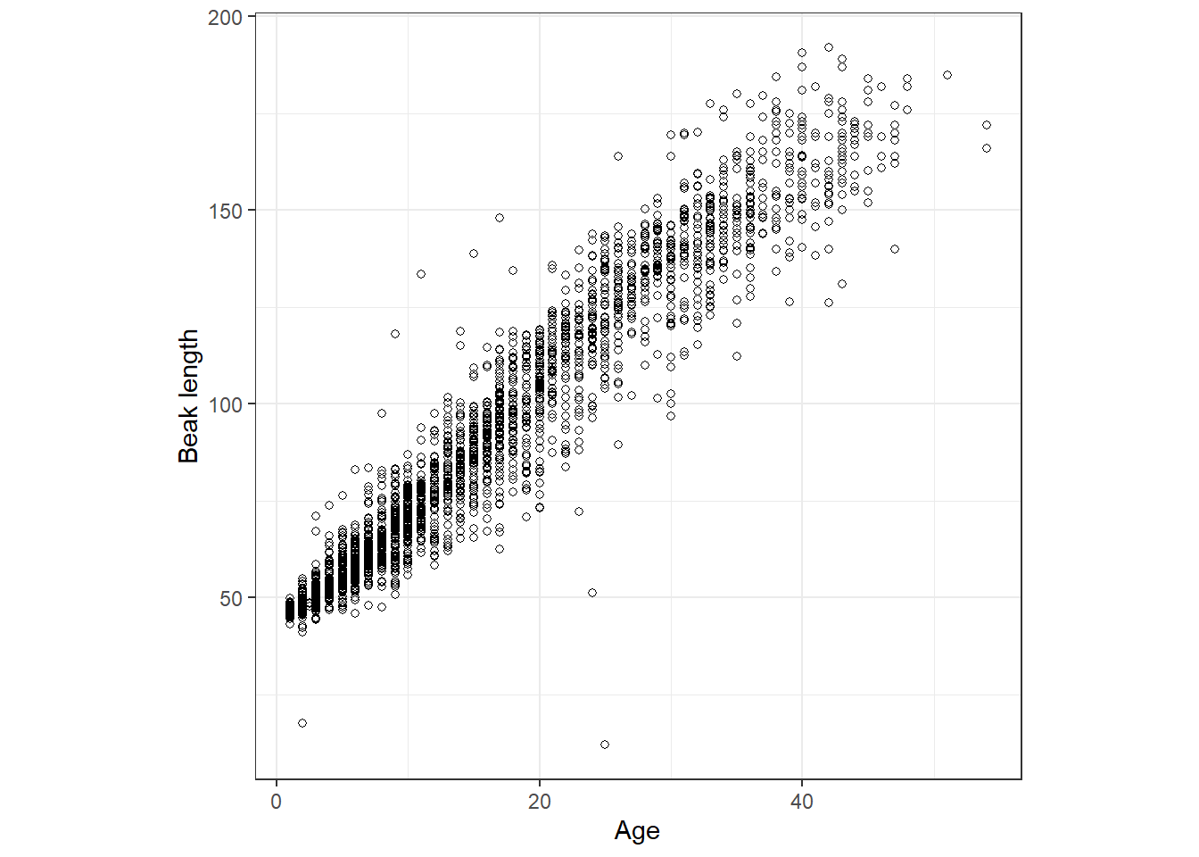
図4.1: Scatterplot of beak length (mm) of White Stork chicks versus age (in days).
4.2 Considering the data (wrongly) as one-way nested
まず、以下のモデルを考える(回帰係数は省略している)。BLはくちばし長、Ageは日齢、Chickは雛のID、Nestはそのデータが得られた巣のIDを表す。
\[ \begin{aligned} BL_i &= Intercept + Age_i + Nest_i + Chick_i + \epsilon_i \\ \epsilon_i &\sim N(0, \sigma^2) \end{aligned} \]
このモデルには2つの大きな問題がある。
- 巣IDと雛IDは多いので、モデルで膨大なパラメータを推定することになる。
- 同じ雛/巣から複数のデータが収集されており、疑似反復が生じている。
この問題を解決する方法として、巣ごとの平均をとることができるがサンプルサイズが著しく減少する。また、巣ごとの平均くちばし長というのは生物学的に見て意味のあるものだとは思えない。混合mドエルはこれらの問題を解決する。
4.2.1 model formulation
まずは、以下の混合モデルを考える。このモデルは、雛IDについてはひとまず無視し、巣IDをランダム切片として含めている。なお、\(i\)は巣IDを表し、\(j = 1,2,3,\dots,n_i\)は巣ごとのデータ数を表す。ここでは、\(a_i\)と\(\epsilon_{ij}\)は独立であると仮定されている。
\[ \begin{aligned} BL_{ij} &= Intercept + Age_{ij} + a_i + \epsilon_{ij} \\ a_i &\sim N(0, \sigma_{nest}^2)\\ \epsilon_{ij} &\sim N(0, \sigma^2) \end{aligned} \]
このモデルは、以下のようにも書ける。
\[
\begin{aligned}
BL_{ij} &= N(\mu_{ij}, \sigma^2)\\
E(BL_{ij}) &= \mu_{ij} \;\; and \;\; var(BL_{ij}) = \sigma^2 \\
\mu_{ij} &= Intercept + Age_{ij} + a_i \\
a_i &\sim N(0, \sigma_{nest}^2)\\
\end{aligned}
\tag{4.1}
\]
生態学では、一元配置入れ子モデル(one-way nested model)の線形混合効果モデルと呼ばれる。それでは、混合モデルはどのようにデータの非独立性に対応しているのだろうか。
同じ巣の雛同士は、同じ親に育てられ、生息環境が同じであり、遺伝的にも類似している。よって、同じ巣の雛のくちばし長は独立ではなく、他の巣の雛のくちばし長よりも類似していると考えられる。
同じ巣の雛のくちばし長同士の相関は、この混合モデルでは以下のように書ける。これは級内相関係数(inter class correlation: ICC)とも呼ばれる。なお、このモデルでは異なる巣の雛のくちばし長同士の相関は0であると仮定される。混合モデルでは、このように巣内のデータの非独立性が考慮される。
\[ cor(BL_{ij}, BL_{ik}) = \phi = \frac{\sigma_{nest}^2}{\sigma_{nest}^2 + \sigma^2} \tag{4.2} \]
巣1(データ数が6)のデータの相関行列は以下のように書ける。
\[
\bf{\Sigma_1} = cor
\begin{pmatrix}
BL_{1,1}\\
BL_{1,2}\\
BL_{1,3}\\
BL_{1,4}\\
BL_{1,5}\\
BL_{1,6}\\
\end{pmatrix} =
\begin{pmatrix}
1 & \phi & \phi & \phi & \phi & \phi \\
\phi & 1 & \phi & \phi & \phi & \phi \\
\phi & \phi & 1 & \phi & \phi & \phi \\
\phi & \phi & \phi & 1 & \phi & \phi \\
\phi & \phi & \phi & \phi & 1 & \phi \\
\phi & \phi & \phi & \phi & \phi & 1 \\
\end{pmatrix}
\]
他の巣についても同じように書ける(データ数に応じて行列数が変わるだけである)。よって、全ての巣のデータの相関係数は以下のように書ける。なお、\(n_1, n_2, \dots, n_{73}\)は各巣のデータ数である。以上で見たように、同じ巣のデータ同士の相関は\(\phi\)、異なる巣のデータ同士の相関は0であると仮定される。
\[ \begin{aligned} cor \begin{pmatrix} \begin{pmatrix} BL_{1,1}\\ \vdots\\ BL_{1,n_1} \end{pmatrix}\\ \begin{pmatrix} BL_{2,1}\\ \vdots\\ BL_{2,n_2} \end{pmatrix}\\ \vdots \\ \begin{pmatrix} BL_{73,1}\\ \vdots\\ BL_{73,n_{73}} \end{pmatrix} \end{pmatrix} = \begin{pmatrix} \bf{\Sigma_1} & 0 & \cdots & 0\\ 0 & \bf{\Sigma_2} & \cdots & 0\\ \vdots & \vdots & \ddots & \vdots \\ 0 & 0 & \cdots & \bf{\Sigma_{73}} \\ \end{pmatrix} \end{aligned} \]
なお、式(4.2)は一つのランダム切片を持つ線形混合モデルについてのみ当てはまる。一般化線形混合モデル(GLMM)や2つ以上のランダム切片/ランダム傾きをもつ線形混合モデルについては異なる表現が用いられる。
混合モデルはGLSと同様にデータ間の相関をモデルに組み込むことによって、データの非独立性に対処している。なお、ランダム切片の分散\(\sigma_{nest}^2\)について正確な推定を行うためには、少なくとも5以上のクラスター(今回の場合は巣ID)がなくてはならない。
4.3 Fitting the one-way nested model using lmer
それでは、モデル(4.1)をRで実行する。ここでは、lme4パッケージのlmer関数を用いる。分析には2012年のデータのみを用いる。
ws2 <- drop_na(ws, beak, age, nest, chick) %>%
  mutate(fnest = as.factor(nest),
         fchick = as.factor(chick)) %>%
  filter(year == "2012") %>%
  data.frame()

m5_1 <- lmer(beak ~ age + (1|fnest),
             data = ws2)
結果は以下の通り。
## Linear mixed model fit by REML ['lmerMod']
## Formula: beak ~ age + (1 | fnest)
##    Data: ws2
##
## REML criterion at convergence: 10234.3
##
## Scaled residuals:
##     Min      1Q  Median      3Q     Max
## -4.9103 -0.5406 -0.0259  0.5768  6.3796
##
## Random effects:
##  Groups   Name        Variance Std.Dev.
##  fnest    (Intercept) 57.23    7.565
##  Residual             62.50    7.905
## Number of obs: 1438, groups:  fnest, 73
##
## Fixed effects:
##             Estimate Std. Error t value
## (Intercept)  44.4417     0.9651   46.05
## age           2.9925     0.0169  177.08
##
## Correlation of Fixed Effects:
##     (Intr)
## age -0.301モデルの結果から、モデル式は以下のように推定されたことが分かる。2行目から\(a_i\)を除いた\(\mu_{ij} = 44.44 + 2.99\times Age_{ij}\)の部分はモデルのfixed partと呼ばれ、平均的な巣におけるくちばし長の期待値を表す(ランダム切片を含まないので)。
\[
\begin{aligned}
BL_{ij} &= N(\mu_{ij}, 7.90^2)\\
\mu_{ij} &= 44.44 + 2.99\times Age_{ij} + a_i \\
a_i &\sim N(0, 7.56^2)\\
\end{aligned}
\]
級内相関\(\phi\)は以下のように求められる。
\[
\phi = \frac{7.56^2}{7.56^2 + 7.90^2} = 0.49
\]
Rでは以下のように求める。よって、同じ巣内のデータ同士の相関は0.47と推定されたことが分かる。
sigma_ranef <- VarCorr(m5_1) %>% as.data.frame() %>% .[1,5]

sigma_ranef^2/(sigma_ranef^2 + sigma(m5_1)^2)
## [1] 0.4780135fixed partの予測値と95%信頼区間を表したのが図4.2である。
nd5_1 <- data.frame(age = seq(min(ws2$age),
                           max(ws2$age),
                           by = 1))

## 説明変数を含む行列
X <- model.matrix(~age, data = nd5_1)

## 予測値と95%信頼区間の算出
fitted5_1 <- nd5_1 %>%
  ## 予測値はbeta × Xで求まる
  mutate(fitted = X %*% fixef(m5_1) %>% .[,1]) %>%
  ## 予測値のseは以下の通り
  mutate(se = sqrt(diag(X %*% vcov(m5_1) %*% t(X)))) %>%
  mutate(ci.low = fitted - 1.96*se,
         ci.high = fitted + 1.96*se)

fitted5_1 %>%
  ggplot(aes(x = age, y = fitted))+
  geom_line()+
  geom_ribbon(aes(ymin = ci.low,
                  ymax = ci.high),
              alpha = 0.2)+
  geom_point(data = ws2,
             aes(y = beak),
             shape =1,
             size = 1.5)+
  theme_bw()+
  theme(aspect.ratio = 1)+
  labs(y = "Beak length", x = "Age")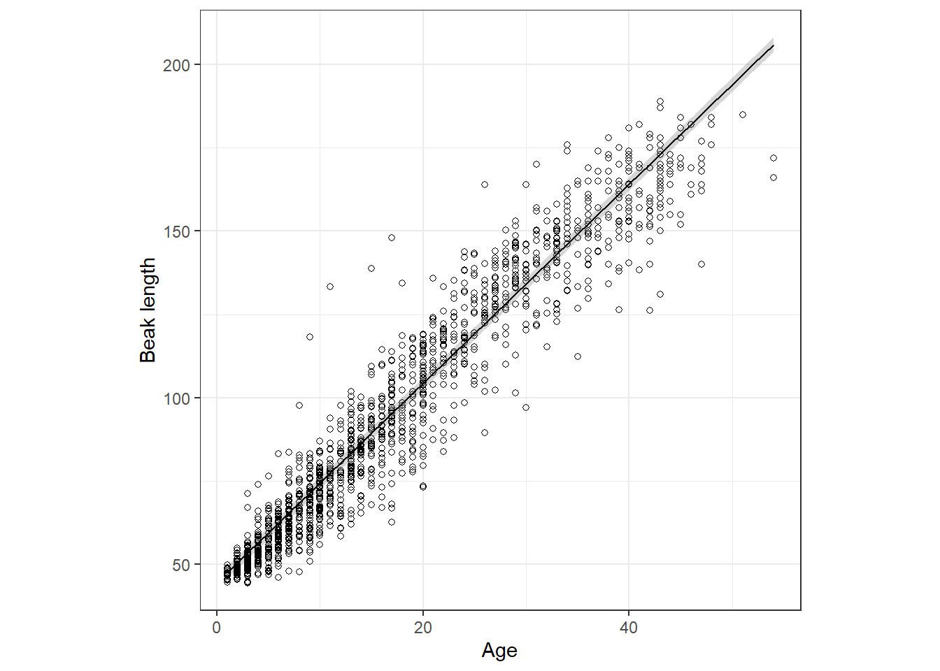
図4.2: Fixed part of the linear mixed-effects model. The shaded area is a 95% confidence interval for the mean.
4.5 Sketching the fitted value
それぞれの巣について推定された\(a_i\)は以下の通り。これは、モデルのrandom partと呼ばれる。
ranef(m5_1) %>%
  data.frame() %>%
  rename(estimated = condval,
         sd = condsd) %>%
  mutate_if(is.numeric, ~round(., 2)) %>%
  datatable()
fixed partとrandom partを足した各巣の予測値を示したのが図4.3である。なお、赤い線は図4.2で示したfixed partのみの直線を示している。それぞれの直線は、ここランダム効果の分だけ上/下にシフトしている。
predict(m5_1) %>%
  data.frame() %>%
  rename(predicted = 1) %>%
  bind_cols(ws2) %>%
  ggplot(aes(x = age))+
  geom_line(aes(y = predicted, group = fnest))+
  geom_point(aes(y = beak),
             shape = 1,size  =1.5)+
    geom_line(data= fitted5_1,
            aes(y = fitted),
            color = "red3",
            linewidth = 1)+
  theme_bw()+
  theme(aspect.ratio = 1)+
  labs(y = "Beak length", x = "Age")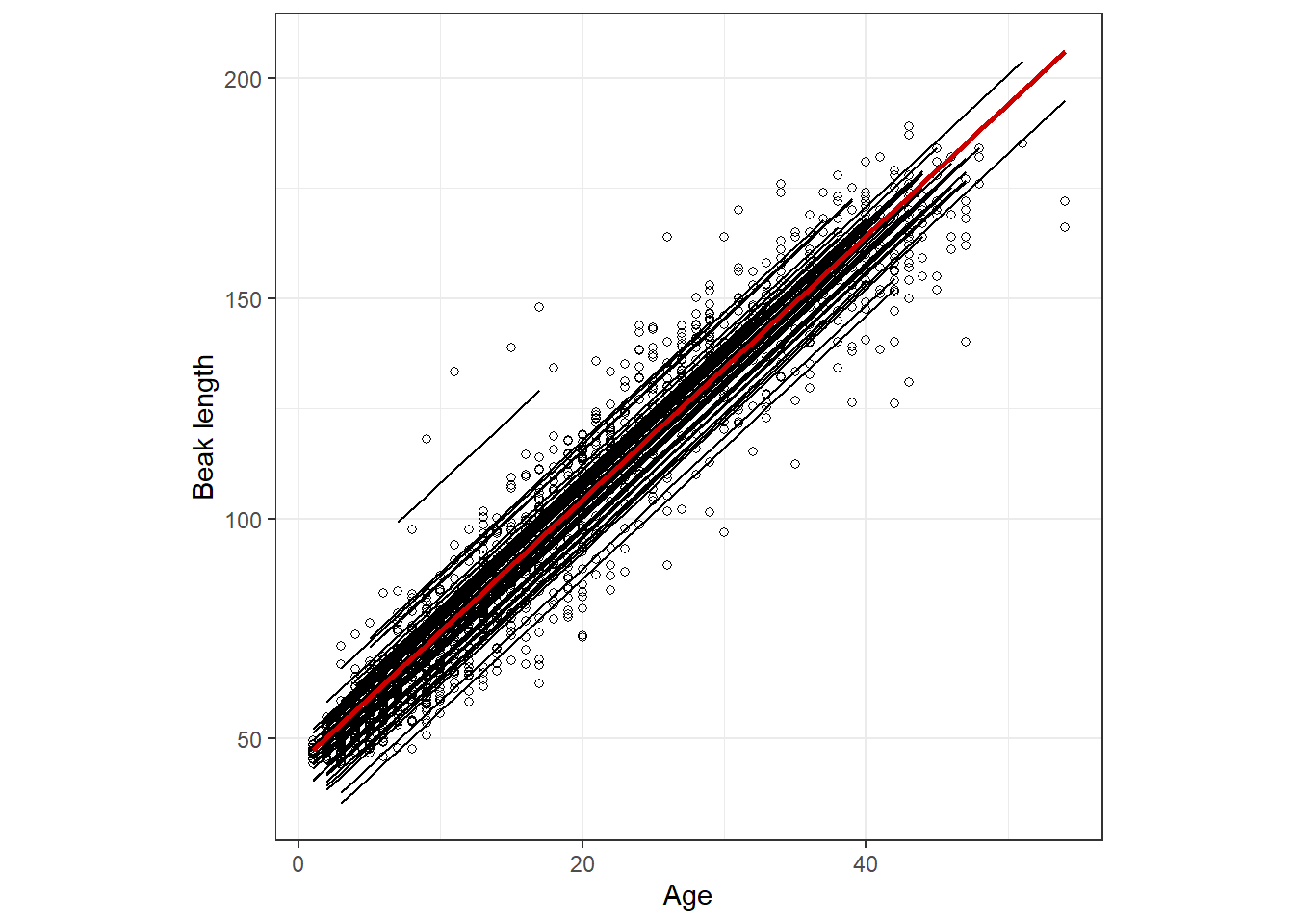
図4.3: Fixed part plus the random effects for the linear mixed-effects model.
4.6 Considering the data (correctly) as two-way nested
さて、それでは次に雛IDも考慮したモデルを考える。データでは同じ雛から複数のデータが収集されており、ここでも疑似反復が生じているからである。同じ雛から得られたデータは、同じ巣の他の雛のデータよりも類似していると考えられる。
以下のようなモデルを考える。このようなモデルは、two-way nested linear mixed-effects modelと呼ばれる。なお、\(i\)は巣IDを、\(j\)は巣ごとの雛IDを、\(k\)は巣\(i\)における\(j\)番目の雛の\(k\)個目のデータであることを表す。
\[ \begin{aligned} BL_{ijk} &= N(\mu_{ijk}, \sigma^2)\\ E(BL_{ijk}) &= \mu_{ijk} \;\; and \;\; var(BL_{ijk}) = \sigma^2 \\ \mu_{ijk} &= Intercept + Age_{ijk} + a_i + b_{ij} \\ a_i &\sim N(0, \sigma_{nest}^2)\\ b_{ij} &\sim N(0, \sigma_{chick}^2)\\ \end{aligned} \tag{4.3} \]
このモデルでは、同じ巣内の異なるデータ間に相関があり、かつ同じ雛の異なるデータ間にも相関があることを仮定している。なお、異なる巣のデータ間は独立だと仮定されている。
同じ巣内の同じ雛のデータ間の相関は以下の式で与えられる。
\[
\phi_{chick} = \frac{\sigma_{nest}^2 + \sigma_{chick}^2}{\sigma_{nest}^2 + \sigma_{chick}^2 + \sigma^2}
\]
また、同じ巣内の異なる雛間のデータの相関は以下の式で表せられる。
\[
\phi_{nest} = \frac{\sigma_{nest}^2}{\sigma_{nest}^2 + \sigma_{chick}^2 + \sigma^2}
\]
このモデルは、Rで以下のように実行できる。
結果は以下の通り。
## Linear mixed model fit by REML ['lmerMod']
## Formula: beak ~ age + (1 | fnest/fchick)
##    Data: ws2
##
## REML criterion at convergence: 9932.6
##
## Scaled residuals:
##     Min      1Q  Median      3Q     Max
## -4.3657 -0.5617 -0.0678  0.5513  6.9810
##
## Random effects:
##  Groups       Name        Variance Std.Dev.
##  fchick:fnest (Intercept) 29.70    5.449
##  fnest        (Intercept) 47.81    6.915
##  Residual                 40.81    6.388
## Number of obs: 1438, groups:  fchick:fnest, 262; fnest, 73
##
## Fixed effects:
##             Estimate Std. Error t value
## (Intercept) 44.41110    0.93656   47.42
## age          2.97532    0.01406  211.63
##
## Correlation of Fixed Effects:
##     (Intr)
## age -0.245iccはそれぞれ\(phi_{chick} = 0.66\)、\(phi_{nest} = 0.40\)と推定された。
sigma_chick <- VarCorr(m5_2) %>% as.data.frame() %>% .[1,5]
sigma_nest <-  VarCorr(m5_2) %>% as.data.frame() %>% .[2,5]
sigma <- sigma(m5_2)

## phi_nest
sigma_nest^2/(sigma^2 + sigma_chick^2 + sigma_nest^2)
## [1] 0.4040858## [1] 0.6550681モデルの結果を図示したのが図4.4である。黒い線はモデルの fixed partの予測値を、赤い点線は巣6(Ap2)の予測値(\(\mu_{ijk} + a_i\))を示している。また、2本の赤い直線は巣6の雛2頭の予測値(\(\mu_{ijk} + a_i + b_{ij}\))を、赤い点はその2頭のデータを示している。これを見ると、2頭の雛の予測値は巣の予測値から近いことが分かる。これは、雛IDのランダム切片よりも巣IDのランダム切片の方が予測値への影響が大きいことを示している。\(\phi_{chick}\)と\(\phi_{nest}\)の値が近いほどこのことがいえる。
re_Ap2 <- ranef(m5_2)$fnest[6,1]

fitted5_2_fixed <- ggpredict(m5_2,
                             terms = "age[1:54,by=0.1]",
                             type = "fixed") %>%
  rename(age = x) %>%
  mutate(fitted_Ap2 = predicted + re_Ap2)

fitted5_2 <- predict(m5_2) %>%
  data.frame() %>%
  bind_cols(ws2) %>%
  rename(fitted = 1)


fitted5_2_fixed %>%
  ggplot(aes(x = age, y = predicted))+
  geom_line(linewidth = 1)+
  geom_line(aes(y = fitted_Ap2),
            data = . %>% filter(age >= 6 & age <= 29),
            linewidth = 0.8, color = "red3",
            linetype = "dashed")+
  geom_line(data = fitted5_2 %>% filter(fnest== "Ap2"),
            aes(y = fitted, group = fchick),
            color = "red3", linewidth = 1)+
  geom_point(data = ws2,
             aes(y = beak),
             shape = 1, size = 1) +
  geom_point(data = ws2 %>% filter(fnest == "Ap2"),
             aes(y = beak, shape = fchick),
             size = 4, color = "red3")+
  scale_shape_manual(values = c(16,18))+
  theme_bw()+
  theme(aspect.ratio = 1)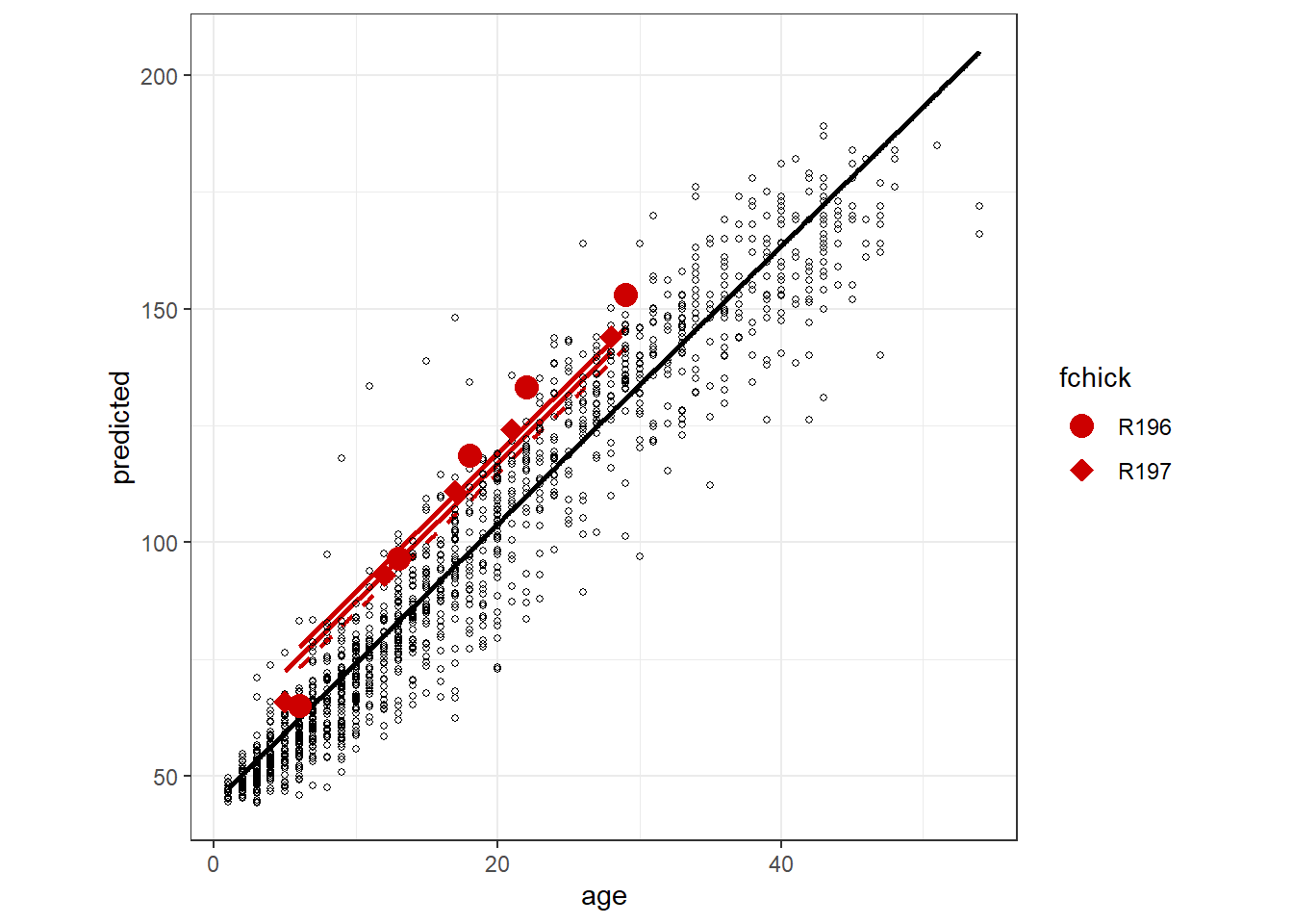
図4.4: Fitted values due to the fixed part, fixed part + the random intercept Nest, and fixed part + the random intercept Nest + the random intercept Chick.
one-way nested model とtwo-way nested model を比較するとパラメータの推定値と標準偏差がわずかに違う。AICを用いてどちらが良いかを調べることもできるが、疑似反復が解消されているtwo-way nested modelを選ぶべきである。
compare_parameters(m5_1, m5_2, select = "{estimate}<br>({se})|{p}") %>%
  data.frame() %>%
  mutate_if(is.numeric, ~round(.,2)) %>%
  select(1,4,5,12,13)
4.7 Differences with the AR1 process approach
第2章で見たような残差AR1過程モデルは残差に時間的な相関があると仮定して疑似反復に対処したが、必ずしも応答変数に時間的相関を仮定したわけではなかった。一方で、混合モデルは応答変数に従属構造があることを考慮して疑似反復に対処している。