9 Poisson, negative binomial, binomial and g amma GLMs in R-INLA
本章では、ポワソン分布、負の二項分布、二項分布、そしてガンマ分布の一般化線形モデル(GLM: generalized linea model)をINLAで行う方法を学ぶ。
9.1 Poisson and negative binomial GLMs in R-INLA
9.1.1 Introduction
本節では、ブラジルに生息するトラギスという魚の体表にいる寄生虫の数を分析した Timi et al. (2008) の研究データを用いる。魚のサンプルはアルゼンチンの3つの海域で採集された(Location)。また、性別(SEX)、体長(LT)、重さ(Weight)、矢状長(LS)が測定されている。LocationとSexは因子型に変換しておく。
sp <- read_delim("data/Turcoparasitos.txt") %>%
  mutate(fSex = as.factor(SEX),
         fLoc = as.factor(Location))

datatable(sp,
          options = list(scrollX = 20),
          filter = "top")
9.1.2 Data exploration
まずはデータの確認を行う。変数のdotplotを見たところ、そこまで極端な外れ値はないよう。
sp %>%
  mutate(n = 1:n()) %>%
  pivot_longer(2:7) %>%
  ggplot(aes(x = value, y = n))+
  geom_point()+
  facet_rep_wrap(~name, repeat.tick.labels = TRUE,
                 scales = "free")+
  labs(y = "Sample number")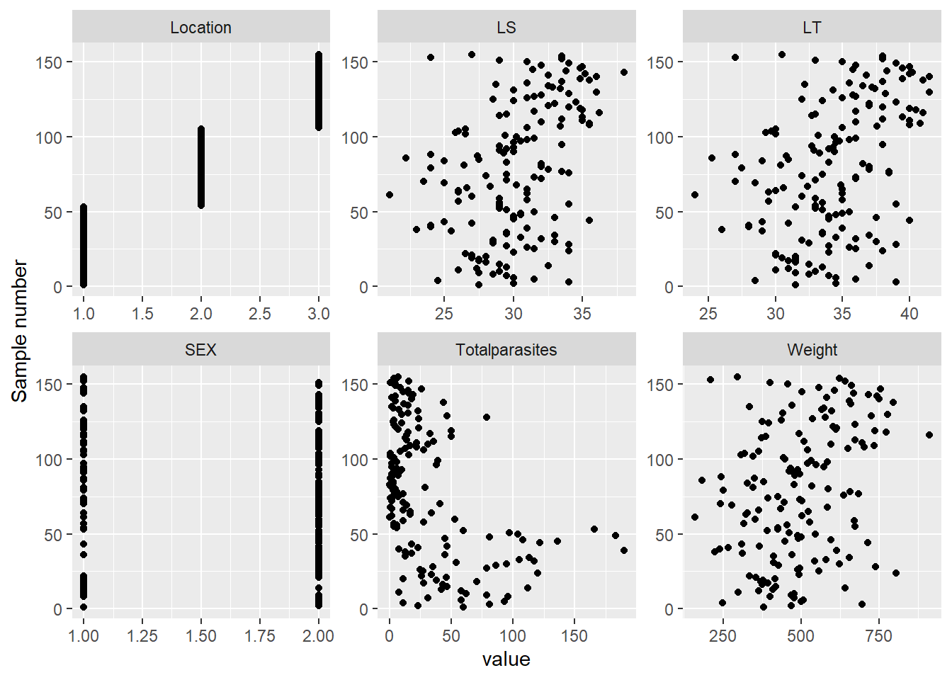
続いて、変数間の関係を確認してみる。体重と体長、矢状長はかなり強く相関しており、これらを同じモデルで使うのは望ましくない。本節では、体長のみを用いる。
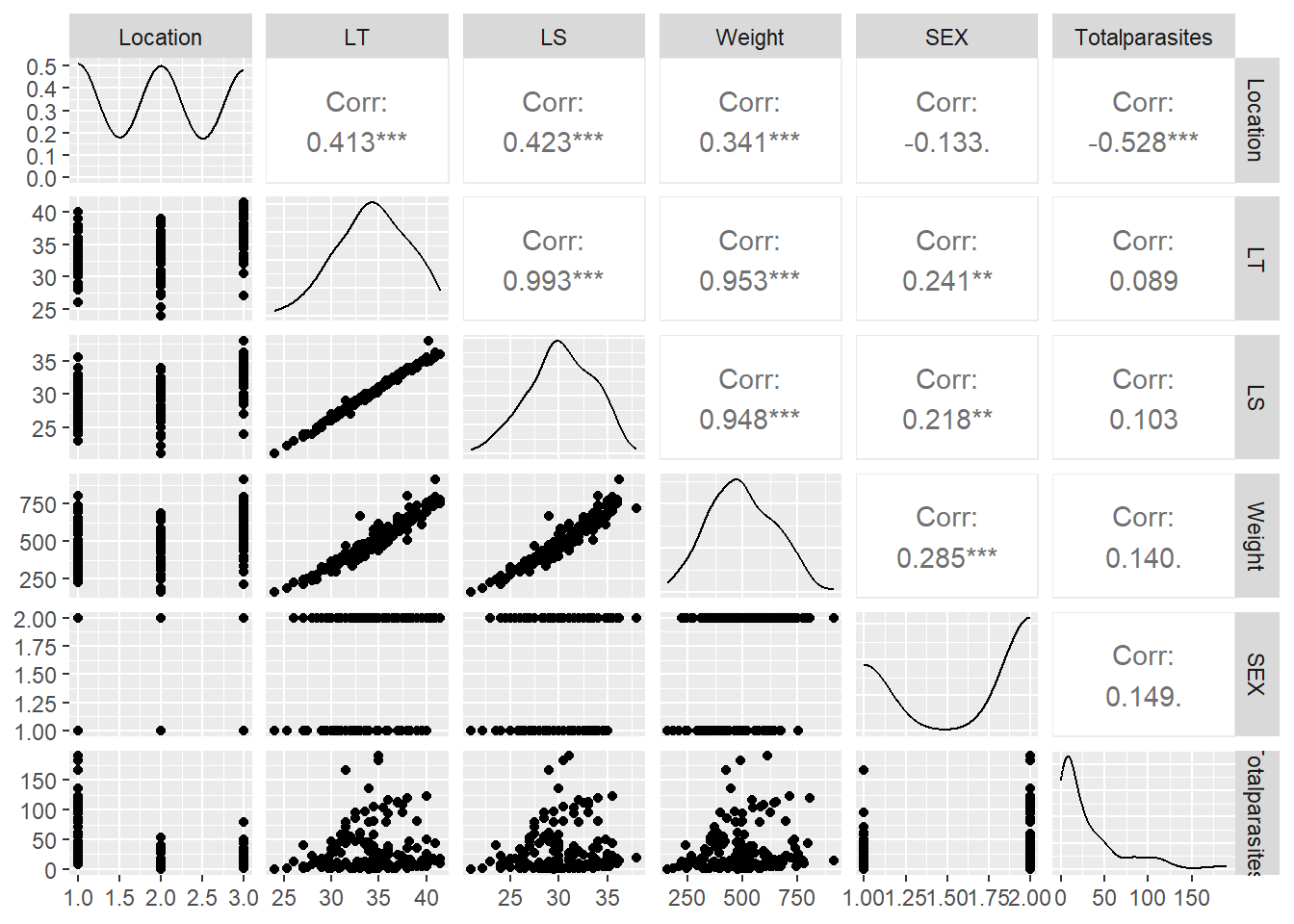
図9.1は海域(Location)ごとに体長と寄生虫の数の関連をプロットしたものである。曲線はポワソン分布のGLMを当てはめたものである。明らかに海域によって傾向が違うことが分かる。つまり、モデルには体長と海域の交互作用を入れる必要がある。
sp %>%
  ggplot(aes(x = LT, y = Totalparasites))+
  geom_point(shape = 1)+
  theme_bw()+
  theme(aspect.ratio = 1)+
  facet_rep_wrap(~Location)+
  geom_smooth(method = "glm",
              method.args = list(family = "poisson"))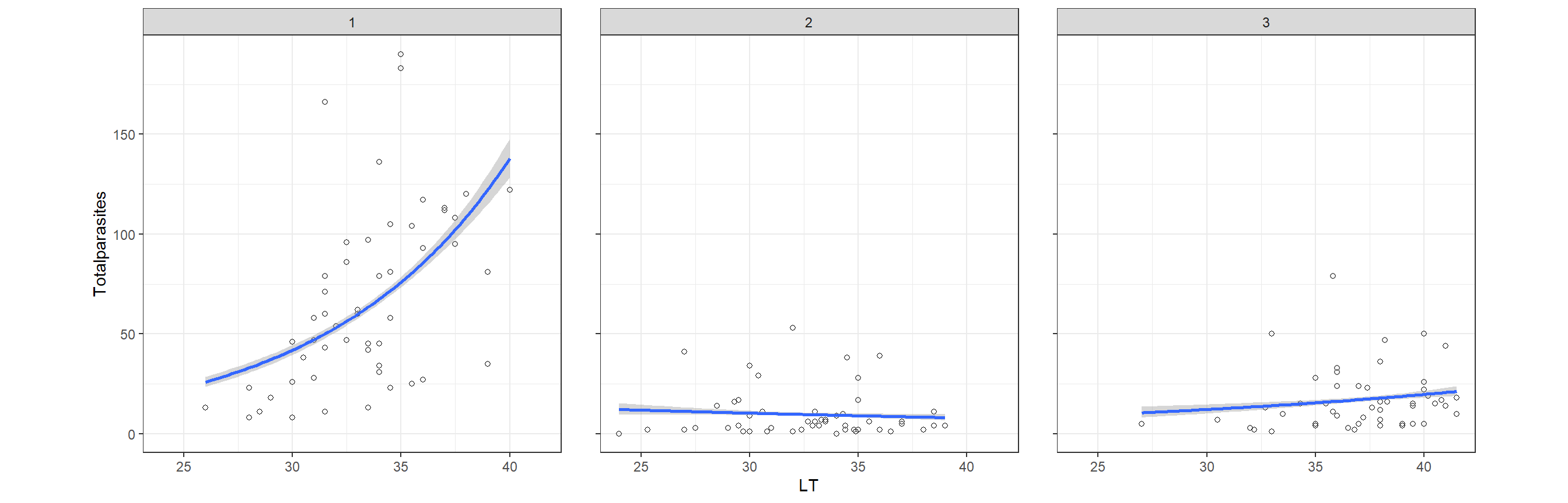
図9.1: Scatterplot of total number of parasites per fish plotted versus length of the fish. Each pane l corresponds to a location.
性別でも見てみたが、こちらはそこまで明確ではない(図9.2)。よって、性別については交互作用を考慮しないこととする。
sp %>%
  ggplot(aes(x = LT, y = Totalparasites))+
  geom_point(shape = 1)+
  theme_bw()+
  theme(aspect.ratio = 1)+
  facet_rep_wrap(~ SEX)+
  geom_smooth(method = "glm",
              method.args = list(family = "poisson"))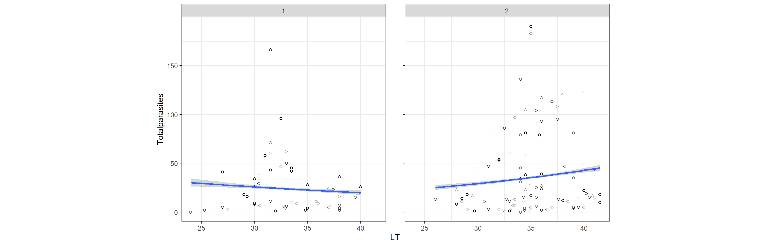
図9.2: Scatterplot of total number of parasites per fish plotted versus length of the fish. Each pane l corresponds to sex.
9.1.3 Poisson GLM an R-INLA
以上から、以下のモデルを考える。\(TP_i\)は寄生虫の数である。なお、回帰係数は省いている。
\[ \begin{aligned} &TP_i \sim Poisson(\mu_i) \\ &E(TP_i) = \mu_i \; and \; var(TP_i) = \mu_i\\ &log(\mu_i) = Intercept + Sex_i + LT_i + Location_i + LT_i \times Location_i \end{aligned} \]
INLAでは以下のように実行できる。
m10_1 <- inla(Totalparasites ~ fSex + LT*fLoc,
              family = "poisson",
              control.compute = list(dic = TRUE),
              data = sp)
結果は以下の通り。
##
## Call:
##    c("inla.core(formula = formula, family = family, contrasts = contrasts,
##    ", " data = data, quantiles = quantiles, E = E, offset = offset, ", "
##    scale = scale, weights = weights, Ntrials = Ntrials, strata = strata,
##    ", " lp.scale = lp.scale, link.covariates = link.covariates, verbose =
##    verbose, ", " lincomb = lincomb, selection = selection, control.compute
##    = control.compute, ", " control.predictor = control.predictor,
##    control.family = control.family, ", " control.inla = control.inla,
##    control.fixed = control.fixed, ", " control.mode = control.mode,
##    control.expert = control.expert, ", " control.hazard = control.hazard,
##    control.lincomb = control.lincomb, ", " control.update =
##    control.update, control.lp.scale = control.lp.scale, ", "
##    control.pardiso = control.pardiso, only.hyperparam = only.hyperparam,
##    ", " inla.call = inla.call, inla.arg = inla.arg, num.threads =
##    num.threads, ", " blas.num.threads = blas.num.threads, keep = keep,
##    working.directory = working.directory, ", " silent = silent, inla.mode
##    = inla.mode, safe = FALSE, debug = debug, ", " .parent.frame =
##    .parent.frame)")
## Time used:
##     Pre = 0.732, Running = 0.471, Post = 0.0719, Total = 1.27
## Fixed effects:
##               mean    sd 0.025quant 0.5quant 0.975quant   mode kld
## (Intercept)  0.171 0.202     -0.224    0.171      0.567  0.171   0
## fSex2        0.008 0.036     -0.063    0.008      0.079  0.008   0
## LT           0.119 0.006      0.107    0.119      0.131  0.119   0
## fLoc2        2.977 0.462      2.071    2.977      3.883  2.977   0
## fLoc3        0.892 0.484     -0.057    0.892      1.840  0.892   0
## LT:fLoc2    -0.146 0.014     -0.173   -0.146     -0.118 -0.146   0
## LT:fLoc3    -0.071 0.013     -0.096   -0.071     -0.045 -0.071   0
##
## Deviance Information Criterion (DIC) ...............: 2752.51
## Deviance Information Criterion (DIC, saturated) ....: 2057.57
## Effective number of parameters .....................: -128.12
##
## Marginal log-Likelihood:  -1552.05
##  is computed
## Posterior summaries for the linear predictor and the fitted values are computed
## (Posterior marginals needs also 'control.compute=list(return.marginals.predictor=TRUE)')この結果から、\(log(\mu_i)\)は以下のように書ける。
\[
\begin{aligned}
log(\mu_i) =
\begin{cases}
0.171 + 0.119 \times LT_i \;\;\;\;\;\;\;\;\;\;\;\;\;\;\;\;\;\;\;\;\;\;\;\;\;\;\;\;\;\;\;\;\;\;\;\;\;\;\;\;\;\;\;\;\; \rm{for \; location = 1, Sex = 1}\\
0.171 + 2.977 + (0.119 - 0.146) \times LT_i \;\;\;\;\;\;\;\;\;\;\;\;\;\;\;\;\; \rm{for \; location = 2, Sex = 1}\\
0.171 + 0.892 + (0.119 - 0.071) \times LT_i \;\;\;\;\;\;\;\;\;\;\;\;\;\;\;\;\; \rm{for \; location = 3, Sex = 1}\\
0.171 + 0.008 + 0.119 \times LT_i \;\;\;\;\;\;\;\;\;\;\;\;\;\;\;\;\;\;\;\;\;\;\;\;\;\;\;\;\;\;\;\; \rm{for \; location = 1, Sex = 2}\\
0.171 + 0.008 + 2.977 + (0.119 - 0.146) \times LT_i \;\;\;\; \rm{for \; location = 2, Sex = 2}\\
0.171 + 0.008 + 0.892 + (0.119 - 0.071) \times LT_i \;\;\;\; \rm{for \; location = 3, Sex = 2}
\end{cases}
\end{aligned}
\]
9.1.3.1 Checking overdispersion
9.1.3.1.1 Calculating dispersion parameter
モデル選択やモデルの解釈に移る前に、まずはこのデータに対してポワソン分布が適切かを確認する。過分散の有無を確認するため、分散パラメータを算出する。分散パラメータ\(\phi\)は以下のように計算できる。なお、\(N\)はサンプル数、\(k\)はパラメータ数である。もし\(\phi\)が1を超えていれば過分散が生じており、1以下であれば過少分散である。通常、\(\phi = 1.5\)くらいまでであれば問題ないと判断される(健太郎 2010)。
\[ \begin{aligned} &E_i = \frac{TP_i - E(TP_i)}{\sqrt{var(TP_i)}}\\ &\phi = \frac{\sum_{i=1}^k E_i^2}{N - k} \end{aligned} \]
Rでは以下のように算出できる。分散パラメータは18.19であり、明らかに過分散が生じている。
mu <- m10_1$summary.fitted.values$mean
E <- (sp$Totalparasites - mu)/sqrt(mu)

N <- nrow(sp)
p <- nrow(m10_1$summary.fixed)

phi <- sum(E^2)/(N-p)

phi
## [1] 18.185849.1.3.1.2 Bayesian method for looking for over/under-dispersion
ただし、ベイズモデリングの場合、事前分布が無情報ではない場合には分散パラメータがそのまま解釈できない可能性がある。そこで、ベイズモデリングでは異なる方法で確認を行う。
MCMCの場合には、各MCMCサンプルごとにデータをシミュレートして実データと比べることで過分散の検討を行える(Zuur and Ieno 2016)。INLAではMCMCをしていないので、事後分布から新たなデータをシミュレートし、これを実測値と比較することで過分散がないかを確認する。具体的には、以下の手順を行う。
INLAでGLMを実行する。
- 事後分布から1セットの回帰係数\(\beta_1, \dots, \beta_7\)をサンプリングする。
- サンプリングしたパラメータを用いて期待値\(\bf{\mu} = exp(\bf{X} \times \bf{\beta})\)を算出する。
- 計算した期待値から
rpois関数を用いてデータをシミュレートする。
- シミュレートしたデータセットのピアソン残差(\(E_i\))を算出し、その平方和(\(\sum_i^N E_i^2\))を計算する。
- 2から5を1000回繰り返す。
- シミュレートしたデータセットのピアソン残差の平方和と実測値のピアソン残差の平方和を比較する。
シミュレートしたデータセットのピアソン残差の平方和の分布は、もしモデルが正しいときにそれに従うデータセットが持つピアソン残差の平方和の分布である。もし過分散/過少分散が生じているのであれば、実際のデータセットのピアソン残差の平方和がこの分布から外れた値をとるはずである。
それでは、実際に行ってみよう。事後分布からパラメータのサンプリングを行うには、control.computeオプションでconfig = TRUEとする必要がある。
m10_2 <- inla(Totalparasites ~ fSex + LT*fLoc,
              family = "poisson",
              control.compute = list(dic = TRUE,
                                     config = TRUE),
data = sp)それでは、パラメータの事後同時分布から1000セットのパラメータをサンプリングする(第7.5.5.2節を参照)。
例えば1セット目にサンプリングされた値は以下の通り。なお、ここでは既にサンプリングしたパラメータを用いた期待値\(\bf{\mu} = exp(\bf{X} \times \bf{\beta})\)も算出されている(最初の155行)。最後の7行はサンプリングされたパラメータの値である。
それでは、抽出した1000セットのパラメータを用いて1000個のデータセットをシミュレートする。
y_sim <- matrix(nrow = nrow(sp),
                ncol = 1000)

for(i in 1:1000){
 y_sim[,i] <- rpois(n = nrow(sp), lambda = exp(sim_param[[i]]$latent[1:nrow(sp),]))
}
続いて、それぞれのデータセットについてピアソン残差の平方和を算出する。
さて、実際に得られた実測値のピアソン残差の平方和は以下の通り、2691.504であった。
## [1] 2691.504これをシミュレートしたデータセットのピアソン残差の平方和と比べると、そのすべてよりも大きいことが分かった。すなわち、実データはデータが想定するよりも非常に大きなばらつきがあるといえる(= 過分散が生じている)。
## [1] 1これは、シミュレートしたでーらセットにおけるピアソン残差の平方和の分布をみても明らかである。モデルに従うのであれば、ピアソン残差の平方和はせいぜい100から300くらいの値しか取らない。
data.frame(x = sum_E2_sim) %>%
  ggplot(aes(x = x)) +
  geom_histogram(binwidth = 5) +
  theme_bw()+
  theme(aspect.ratio = 0.8)
図9.3: シミュレートされたデータのピアソン残差の平方和の分布
過分散はデータのばらつきがポワソン分布が仮定するよりも大きすぎるときのほかに、外れ値の影響や共変量を入れていないこと、交互作用がないことやリンク関数が間違っていること、非線形のパターンがあることやゼロ過剰、データの非独立性などが原因でも起きる。データをしっかりとみて原因に合った解決をしなくてはならない。
今回はゼロ過剰や外れ値の影響はなさそうである。また、予測値とピアソン残差の関係を見ても、明確にパターンがあるわけではなさそう。また、ピアソン残差と共変量の間にパターンもなく、応答変数と説明変数の間に非線形な関係があるというわけでもなさそう。
data.frame(resid = (sp$Totalparasites - mu)/sqrt(mu),
           fitted = m10_2$summary.fitted.values$mean) %>%
  ggplot(aes(x = fitted, y = resid))+
  geom_point()+
  geom_hline(yintercept = 0,
             linetype = "dashed")+
  theme_bw()+
  theme(aspect.ratio = 1)+
  labs(x = "Fitted values",
       y = "Pearson residuals")-> p1

data.frame(resid = (sp$Totalparasites - mu)/sqrt(mu),
           LT = sp$LT) %>%
  ggplot(aes(x = LT, y = resid))+
  geom_point()+
  geom_hline(yintercept = 0,
             linetype = "dashed")+
  theme_bw()+
  theme(aspect.ratio = 1)+
  labs(x = "LT",
       y = "Pearson residuals")-> p2

data.frame(resid = (sp$Totalparasites - mu)/sqrt(mu),
           Loc = sp$fLoc,
           Sex = sp$fSex) %>%
  pivot_longer(2:3) %>%
  ggplot(aes(x = value, y = resid))+
  geom_boxplot()+
  facet_rep_wrap(~name, repeat.tick.labels = TRUE,
                 scales = "free")+
  theme_bw()+
  theme(aspect.ratio = 1)+
  labs(x = "",
       y = "Pearson residuals")-> p3


(p1 + p2)/p3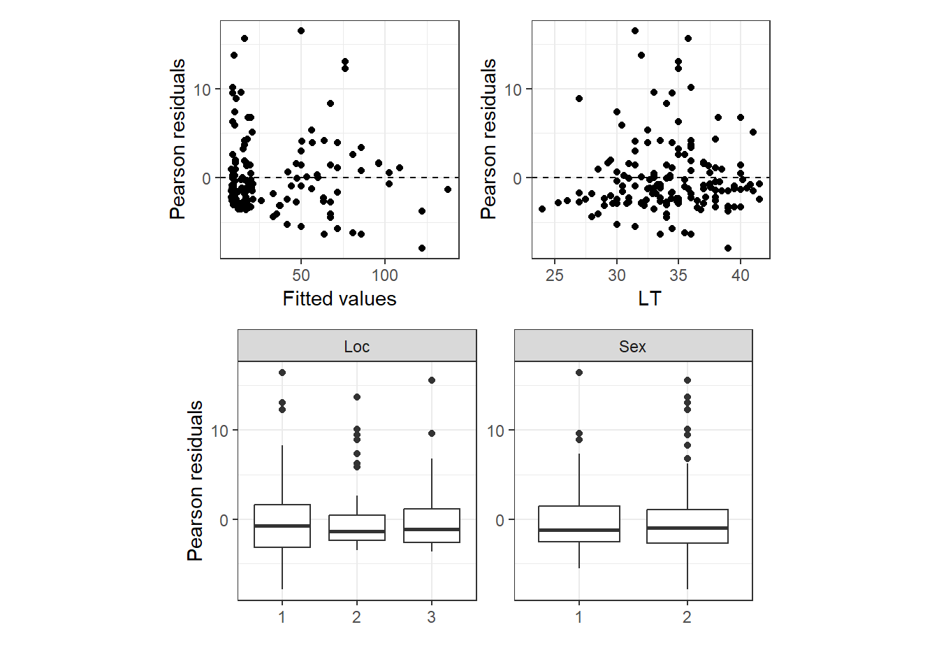
そこで、本節では以下で負の二項分布を適用したモデリングを行う。
9.1.4 Negative binomial GLM in R-INLA
モデル式は以下のとおりである。\(k\)は負の二項分布の分散パラメータで、分布の分散を調整する。INLAではsizeパラメータと呼ばれる。
\[ \begin{aligned} &TP_i \sim NegBinomial(\mu_i, k) \\ &E(TP_i) = \mu_i \; and \; var(TP_i) = \mu_i + \frac{\mu_i^2}{k}\\ &log(\mu_i) = Intercept + Sex_i + LT_i + Location_i + LT_i \times Location_i \end{aligned} \]
INLAでは以下のように実行する。
m10_3 <- inla(Totalparasites ~ fSex + LT*fLoc,
              family = "nbinomial",
              control.compute = list(dic = TRUE,
                                     config = TRUE),
              data = sp)
結果は以下の通り。ポワソンモデルのときと比べて、確信区間が全て広くなっている。
##
## Call:
##    c("inla.core(formula = formula, family = family, contrasts = contrasts,
##    ", " data = data, quantiles = quantiles, E = E, offset = offset, ", "
##    scale = scale, weights = weights, Ntrials = Ntrials, strata = strata,
##    ", " lp.scale = lp.scale, link.covariates = link.covariates, verbose =
##    verbose, ", " lincomb = lincomb, selection = selection, control.compute
##    = control.compute, ", " control.predictor = control.predictor,
##    control.family = control.family, ", " control.inla = control.inla,
##    control.fixed = control.fixed, ", " control.mode = control.mode,
##    control.expert = control.expert, ", " control.hazard = control.hazard,
##    control.lincomb = control.lincomb, ", " control.update =
##    control.update, control.lp.scale = control.lp.scale, ", "
##    control.pardiso = control.pardiso, only.hyperparam = only.hyperparam,
##    ", " inla.call = inla.call, inla.arg = inla.arg, num.threads =
##    num.threads, ", " blas.num.threads = blas.num.threads, keep = keep,
##    working.directory = working.directory, ", " silent = silent, inla.mode
##    = inla.mode, safe = FALSE, debug = debug, ", " .parent.frame =
##    .parent.frame)")
## Time used:
##     Pre = 0.658, Running = 0.168, Post = 0.109, Total = 0.935
## Fixed effects:
##               mean    sd 0.025quant 0.5quant 0.975quant   mode kld
## (Intercept) -1.005 1.452     -3.857   -1.005      1.847 -1.005   0
## fSex2        0.010 0.159     -0.303    0.010      0.323  0.010   0
## LT           0.153 0.044      0.066    0.153      0.240  0.153   0
## fLoc2        4.392 1.910      0.644    4.392      8.144  4.391   0
## fLoc3        1.812 2.126     -2.363    1.812      5.989  1.812   0
## LT:fLoc2    -0.188 0.058     -0.301   -0.188     -0.075 -0.188   0
## LT:fLoc3    -0.099 0.060     -0.217   -0.099      0.019 -0.099   0
##
## Model hyperparameters:
##                                                        mean    sd 0.025quant
## size for the nbinomial observations (1/overdispersion) 1.56 0.186       1.22
##                                                        0.5quant 0.975quant mode
## size for the nbinomial observations (1/overdispersion)     1.55       1.95 1.53
##
## Deviance Information Criterion (DIC) ...............: 1276.63
## Deviance Information Criterion (DIC, saturated) ....: 185.45
## Effective number of parameters .....................: 8.00
##
## Marginal log-Likelihood:  -673.93
##  is computed
## Posterior summaries for the linear predictor and the fitted values are computed
## (Posterior marginals needs also 'control.compute=list(return.marginals.predictor=TRUE)')INLAではsizeパラメータ\(k\)の事前分布は、\(\theta = log(k)\)の事前分布が\(logGamma(1,0.1)\)になるようになっている。\(k\)の事後平均値は1.56であった。事後分布は以下の通り。
m10_3$marginals.hyperpar$`size for the nbinomial observations (1/overdispersion)` %>%
  data.frame() %>%
  ggplot(aes(x = x, y = y))+
  geom_area(fill = "lightblue")+
  geom_line()+
  theme_bw()+
  theme(aspect.ratio = 1)+
  labs(x = expression(k),
       y = expression(paste("Pr(",k,"|D)")))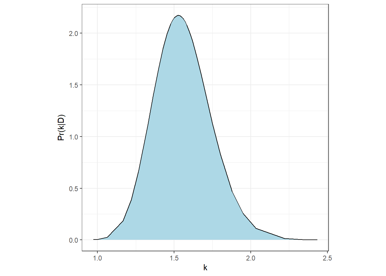
もし\(k\)の値を固定したいときは以下のようにすればよい。モデル選択をする際など\(k\)の値が変わると困る場合に用いればよい。
hyp.nb <- list(size = list(initial = 1,
                           fixed = TRUE))

m10_4 <- inla(Totalparasites ~ fSex + LT*fLoc,
              family = "nbinomial",
              control.compute = list(dic = TRUE,
                                     config = TRUE),
              control.family = list(hyper = hyp.nb),
data = sp)以下では、ポワソン分布のときと同じように過分散のチェックを行う。確認の結果、シミュレーションによって得られたポワソン残差の平方和の分布と実際のポワソン残差の平方和を示したのが図9.4である。実際の平方和はシミュレーションの値の87%より大きいが、ポワソン分布に比べると過分散がかなり改善していることが分かった。
sim_param.nb <- inla.posterior.sample(n = 1000, m10_3)

y_sim.nb <- matrix(nrow = nrow(sp),
                   ncol = 1000)

for(i in 1:1000){
 y_sim.nb[,i] <- rnbinom(n = nrow(sp),
                      mu = exp(sim_param[[i]]$latent[1:nrow(sp),]),
                      size = sim_param.nb[[i]]$hyperpar[[1]])
}

### シミュレートしたデータセットのピアソン残差の平方和
sum_E2_sim.nb <- vector()
mu <- m10_3$summary.fitted.values$mean
k <- m10_3$summary.hyperpar$mean

for(i in 1:1000){
  E <- (y_sim.nb[,i] - mu)/sqrt(mu + mu^2/k)
  sum_E2_sim.nb[i] <- sum(E^2)
}

### 実データのピアソン残差の平方和
E <-(sp$Totalparasites - mu)/sqrt(mu + mu^2/k)
sum_E2.nb <- sum(E^2)

### 比較
p <- mean(sum_E2.nb > sum_E2_sim.nb)

data.frame(x = sum_E2_sim.nb) %>%
  ggplot(aes(x = x)) +
  geom_histogram(binwidth = 5) +
  theme_bw()+
  theme(aspect.ratio = 0.8) +
  geom_vline(xintercept = sum_E2.nb,
             color = "red2")+
  geom_text(aes(x = 210, y = 60),
            label = str_c("p = ", p))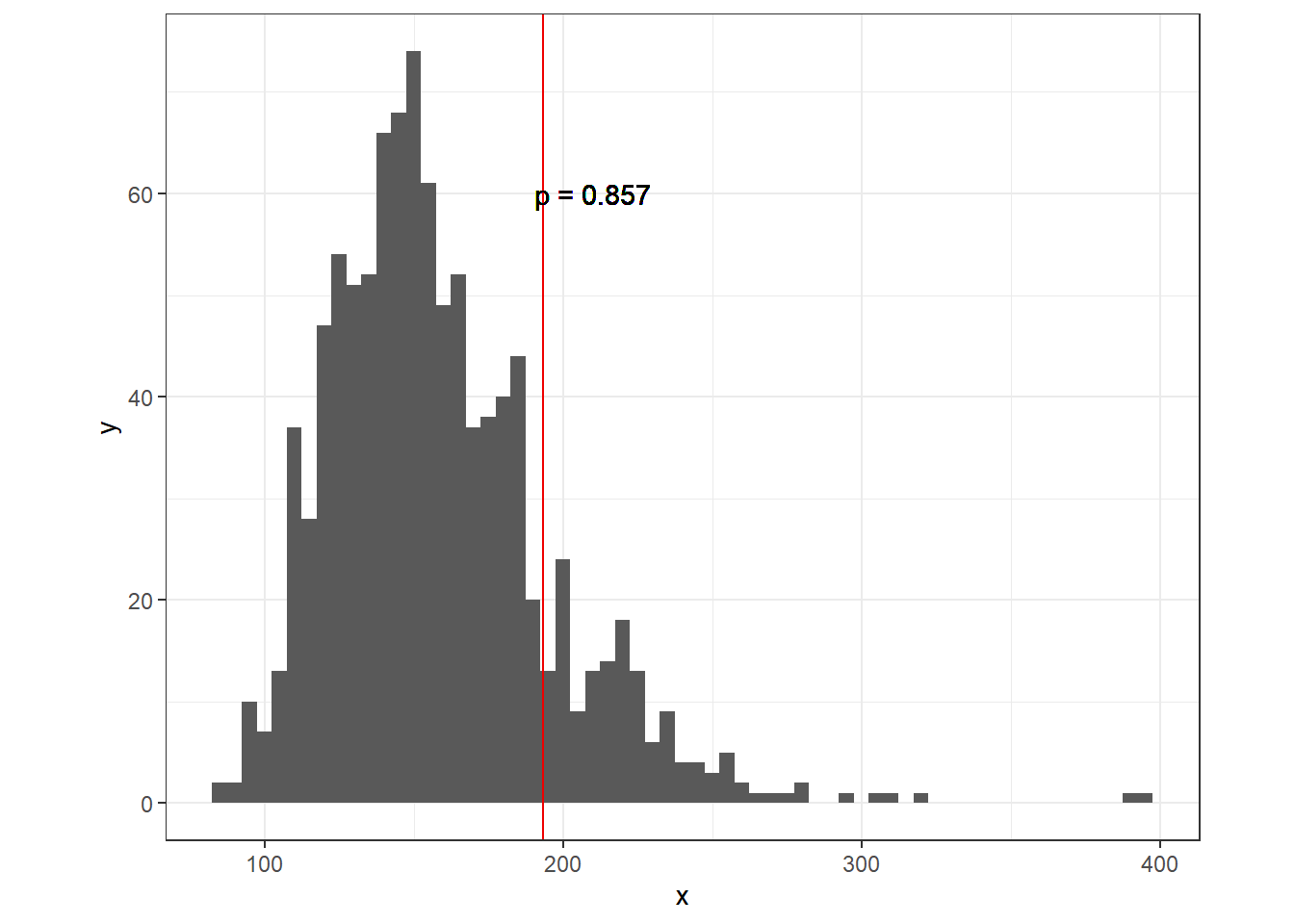
図9.4: シミュレートされたデータのピアソン残差の平方和の分布の実データのピアソン残差の平方和
9.1.5 Model selection for the NB GLM
モデル選択は議論の多い話題ではあるが、以下ではひとまずDICとWAICによるモデル選択を行う。なお、比較のため\(k\)は先ほどのモデルで得られた値に固定する。ひとまず、1つずつ説明変数をなくした場合と比較を行う。
hyper.nb <- list(size = list(initial = k,
                             fixed = TRUE))

## フルモデル
m10_5 <- inla(Totalparasites ~ fSex + LT*fLoc,
              family = "nbinomial",
              control.compute = list(dic = TRUE,
                                     waic = TRUE,
                                     config = TRUE),
              control.family = list(hyper = hyp.nb),
              data = sp)

## fSexなし
m10_5a <- inla(Totalparasites ~  LT*fLoc,
              family = "nbinomial",
              control.compute = list(dic = TRUE,
                                     waic = TRUE,
                                     config = TRUE),
              control.family = list(hyper = hyp.nb),
              data = sp)

## 交互作用項なし
m10_5b <- inla(Totalparasites ~  fSex + LT + fLoc,
              family = "nbinomial",
              control.compute = list(dic = TRUE,
                                     waic = TRUE,
                                     config = TRUE),
              control.family = list(hyper = hyp.nb),
data = sp)まずこれらの3つのモデルでDICとWAICを比較したところ、fSexがないモデルがどちらも最も低いことが分かった。
dic10_5 <- c(m10_5$dic$dic, m10_5a$dic$dic, m10_5b$dic$dic)
waic10_5 <- c(m10_5$waic$waic, m10_5a$waic$waic, m10_5b$waic$waic)

data.frame("type" = c("Full", "-fSex", "-LT × fLoc"),
           DIC = dic10_5,
           WAIC = waic10_5) %>%
  column_as_rownames(var = "type")
最後に、ここから交互作用を除いたモデルと比較を行う。
m10_5c <- inla(Totalparasites ~  LT + fLoc,
              family = "nbinomial",
              control.compute = list(dic = TRUE,
                                     waic = TRUE,
                                     config = TRUE),
              control.family = list(hyper = hyp.nb),
              data = sp)
その結果、やはり交互作用を含むモデルの方がDICとWAICは低い。
dic10_5.2 <- c(m10_5a$dic$dic, m10_5c$dic$dic)
waic10_5.2 <- c(m10_5a$waic$waic, m10_5c$waic$waic)

data.frame("type" = c("Full", "-LT × fLoc"),
           DIC = dic10_5.2,
           WAIC = waic10_5.2) %>%
column_as_rownames(var = "type")以上の結果は、m10_5aが最適なモデルであることを示唆している。このモデルの残差と予測値、残差と共変量の関連を示したのが図@ref(fig:modelvalidation10.5a)である。パターンがあるように見えるが、 Zuur (2017) は問題がなかったと述べている。
mu <- m10_5a$summary.fitted.values$mean
k <- k
resid <- (sp$Totalparasites - mu)/sqrt(mu + mu^2/k)

data.frame(resid = resid,
           fitted = mu) %>%
  ggplot(aes(x = fitted, y = resid))+
  geom_point()+
  geom_hline(yintercept = 0,
             linetype = "dashed")+
  theme_bw()+
  theme(aspect.ratio = 1)+
  labs(x = "Fitted values",
       y = "Pearson residuals")-> p1

data.frame(resid = resid,
           LT = sp$LT) %>%
  ggplot(aes(x = LT, y = resid))+
  geom_point()+
  geom_hline(yintercept = 0,
             linetype = "dashed")+
  theme_bw()+
  theme(aspect.ratio = 1)+
  labs(x = "LT",
       y = "Pearson residuals")-> p2

data.frame(resid = resid,
           Loc = sp$fLoc,
           Sex = sp$fSex) %>%
  pivot_longer(2:3) %>%
  ggplot(aes(x = value, y = resid))+
  geom_boxplot()+
  facet_rep_wrap(~name, repeat.tick.labels = TRUE,
                 scales = "free")+
  theme_bw()+
  theme(aspect.ratio = 1)+
  labs(x = "",
       y = "Pearson residuals")-> p3


(p1 + p2)/p3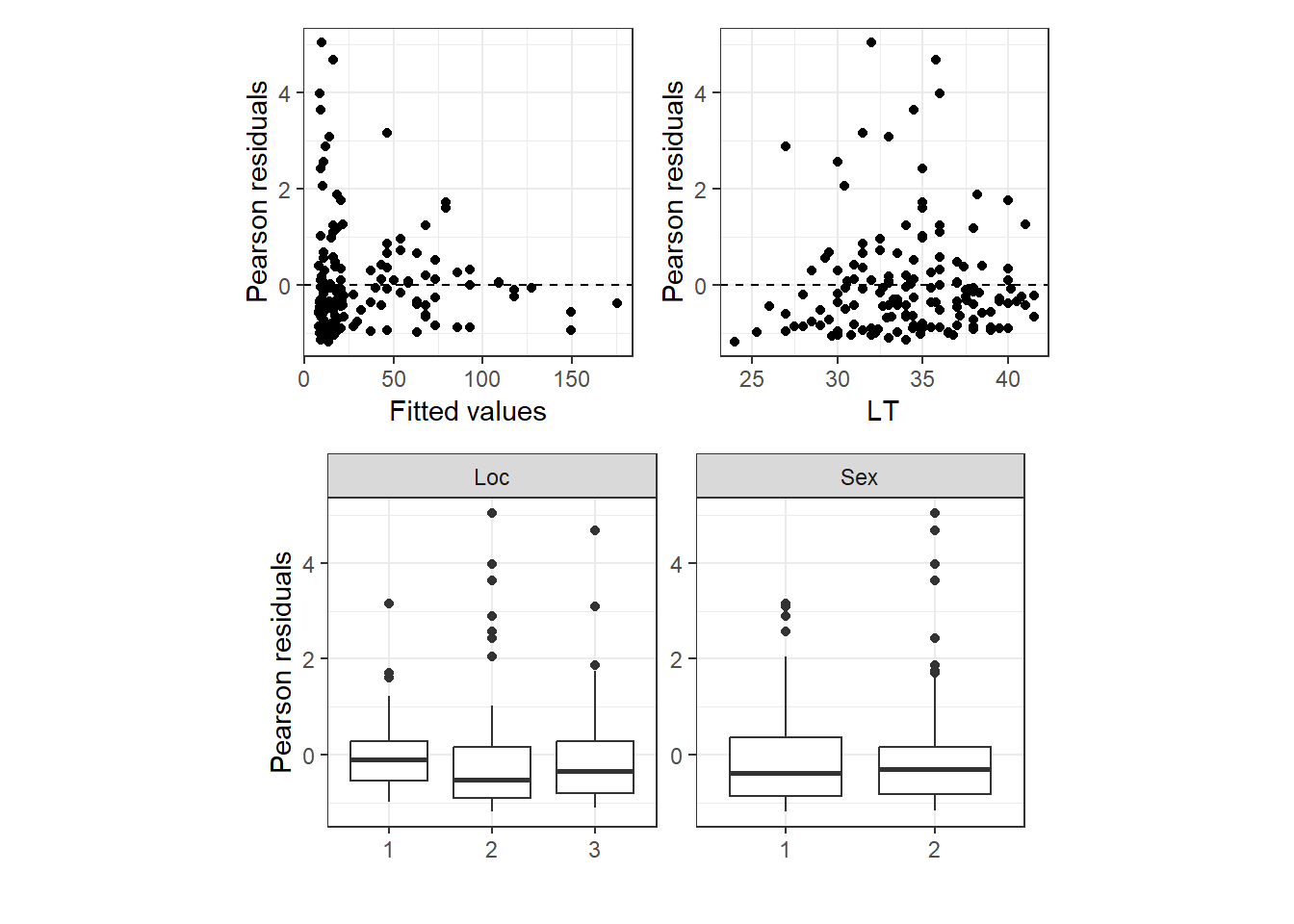
(#fig:modelvalidation10.5a)Model validation for m10_5a
これまで同様に過分散のチェックも行ったが、大きな問題はないよう。
sim_param.nb <- inla.posterior.sample(n = 1000, m10_5a)

y_sim.nb <- matrix(nrow = nrow(sp),
                   ncol = 1000)

for(i in 1:1000){
 y_sim.nb[,i] <- rnbinom(n = nrow(sp),
                      mu = exp(sim_param[[i]]$latent[1:nrow(sp),]),
                      size = k)
}

### シミュレートしたデータセットのピアソン残差の平方和
sum_E2_sim.nb <- vector()
mu <- m10_5a$summary.fitted.values$mean
k <- k

for(i in 1:1000){
  E <- (y_sim.nb[,i] - mu)/sqrt(mu + mu^2/k)
  sum_E2_sim.nb[i] <- sum(E^2)
}

### 実データのピアソン残差の平方和
E <-(sp$Totalparasites - mu)/sqrt(mu + mu^2/k)
sum_E2.nb <- sum(E^2)

### 比較
p <- mean(sum_E2.nb > sum_E2_sim.nb)

data.frame(x = sum_E2_sim.nb) %>%
  ggplot(aes(x = x)) +
  geom_histogram(binwidth = 5) +
  theme_bw()+
  theme(aspect.ratio = 0.8) +
  geom_vline(xintercept = sum_E2.nb,
             color = "red2")+
  geom_text(aes(x = 210, y = 60),
            label = str_c("p = ", p))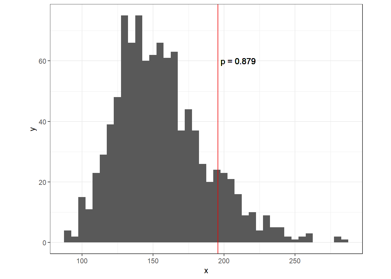
図9.5: シミュレートされたデータのピアソン残差の平方和の分布の実データのピアソン残差の平方和
9.1.6 Visualization of the NB GLM
以下では、結果の可視化を行う。なお、ここでは前章(8.8.2)で用いたinla.make.lincomsを用いる方法で実行する。
まずは予測値が欲しい範囲の変数を格納したデータフレームを作る。
newdata <- crossing(LT = seq(min(sp$LT), max(sp$LT),length =100),
                    fLoc = c("1","2","3"))

X <- model.matrix(~ LT*fLoc, data = newdata) %>%
as.data.frame()次に、lincombsオプションでlcbを指定してモデルを実行する。
lcb <- inla.make.lincombs(X)

m10_6 <- inla(Totalparasites ~  LT*fLoc,
              family = "nbinomial",
              lincomb = lcb,
              control.predictor = list(compute = TRUE),
              control.compute = list(return.marginals.predictor = TRUE),
              control.family = list(hyper = hyper.nb),
data = sp)注意しなければならないのは、m10_6$summary.lincomb.derivedなどは線形予測子、つまり\(log(\mu_i)\)の事後分布についての情報を返してくるということだ。私たちは\(\mu_i\)の予測値が欲しいので、これを変換する必要がある。
以下のようにして変換して事後分布の要約統計量を算出する。
## 線形予測子の事後周辺分布
post_pred10_6 <- m10_6$marginals.lincomb.derived

## 変換を行って要約統計量を計算

## 95%確信区間
ci.10_6 <- map_df(post_pred10_6, ~inla.qmarginal(c(0.025, 0.975),
                                                 inla.tmarginal(exp,.))) %>%
  t() %>%
  as.data.frame() %>%
  rename(lower = 1, upper = 2)

## 事後平均値
mean.10_6 <- map_df(post_pred10_6, ~inla.emarginal(exp,.)) %>%
  t() %>%
  as.data.frame() %>%
  rename(fitted = 1)
結果を図示したのが以下の図である。
## 作図
bind_cols(newdata, ci.10_6, mean.10_6) %>%
  mutate(fLoc = str_c("Location = ", fLoc)) %>%
  ggplot(aes(x = LT, y = fitted))+
  geom_line()+
  geom_ribbon(aes(ymin = lower, ymax = upper),
              alpha = 0.2)+
  geom_point(data = sp %>%
               mutate(fLoc = str_c("Location = ", fLoc)),
             aes(y = Totalparasites),
             shape = 1)+
  facet_rep_wrap(~fLoc, repeat.tick.labels = TRUE)+
  coord_cartesian(ylim = c(0,300))+
  theme_bw()+
  theme(aspect.ratio = 1)+
  labs(y = "Total parasites")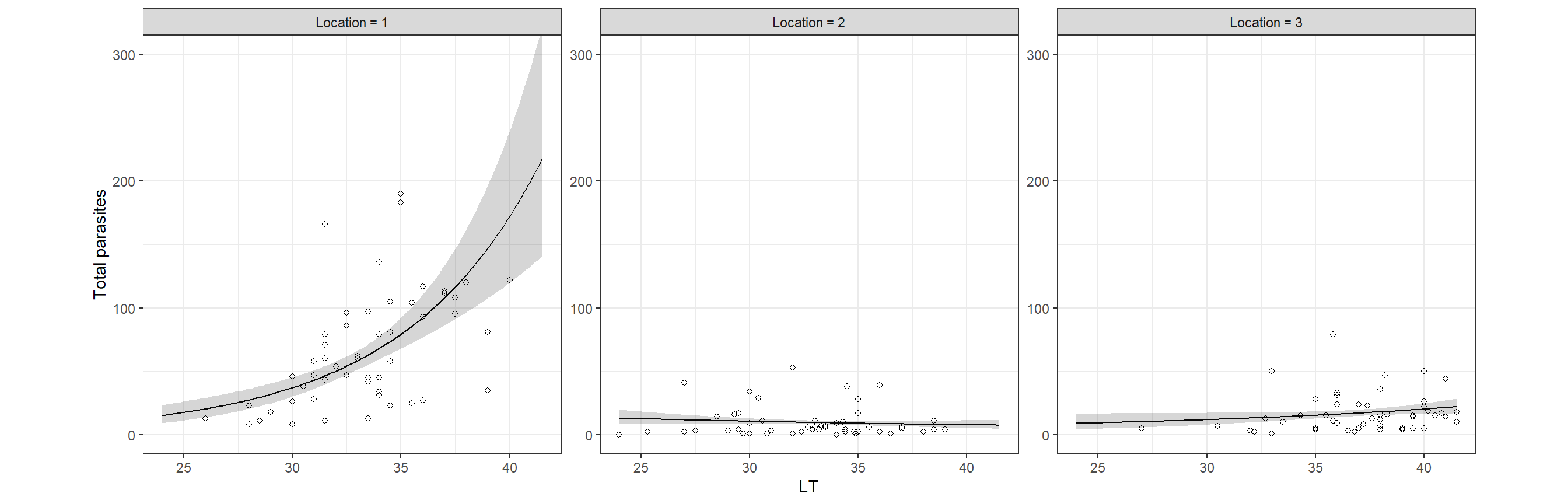
図9.6: Posterior mean fitted values and 95% credible intervals.
9.2 Bernoulli and binomial GLM
本節では、INLAでベルヌーイ分布と二項分布のモデルを実行する方法を学ぶ。
9.2.1 Bernoulli GLM
ここでは、オーストラリアでワニに襲われた人の生死を分析した Fukuda et al. (2015) のデータを用いる。襲われた場所(Position)、ワニと人間の体重の差(DeltaWeight)などの要因が生死(Survival)に与える影響が分析されている。
croco <- read_delim("data/Crocodiles.txt")

datatable(croco,
          options = list(scrollX = 80),
          filter = "top")
ここでは、よりシンプルに考えるため体重差のみを説明変数に入れたモデルを考える。
\[
\begin{aligned}
&Survived_i \sim Bernoulli(\pi_i)\\
&E(Survived_i) = \pi_i \; and \; var(Survived_i) = \pi_i \times (1-\pi_i)\\
&logit(\pi_i) = log \Bigl(\frac{\pi_i}{1 - \pi_i} \Bigl) = \beta_1 + \beta_2 \times DeltaWeight_i
\end{aligned}
\]
Rでは以下のように実行する。応答変数は数字である必要がある。また、ベルヌーイ分布の場合はNtrials = 1となる(なくても実行はできる)。
m10_7 <- inla(Survived01 ~ DeltaWeight,
              data = croco,
              family = "binomial",
              control.predictor = list(compute = TRUE),
              Ntrials = 1)
結果は以下の通り。
##
## Call:
##    c("inla.core(formula = formula, family = family, contrasts = contrasts,
##    ", " data = data, quantiles = quantiles, E = E, offset = offset, ", "
##    scale = scale, weights = weights, Ntrials = Ntrials, strata = strata,
##    ", " lp.scale = lp.scale, link.covariates = link.covariates, verbose =
##    verbose, ", " lincomb = lincomb, selection = selection, control.compute
##    = control.compute, ", " control.predictor = control.predictor,
##    control.family = control.family, ", " control.inla = control.inla,
##    control.fixed = control.fixed, ", " control.mode = control.mode,
##    control.expert = control.expert, ", " control.hazard = control.hazard,
##    control.lincomb = control.lincomb, ", " control.update =
##    control.update, control.lp.scale = control.lp.scale, ", "
##    control.pardiso = control.pardiso, only.hyperparam = only.hyperparam,
##    ", " inla.call = inla.call, inla.arg = inla.arg, num.threads =
##    num.threads, ", " blas.num.threads = blas.num.threads, keep = keep,
##    working.directory = working.directory, ", " silent = silent, inla.mode
##    = inla.mode, safe = FALSE, debug = debug, ", " .parent.frame =
##    .parent.frame)")
## Time used:
##     Pre = 0.592, Running = 0.113, Post = 0.0354, Total = 0.74
## Fixed effects:
##               mean    sd 0.025quant 0.5quant 0.975quant   mode kld
## (Intercept)  2.760 0.516      1.748    2.760      3.772  2.760   0
## DeltaWeight -0.017 0.003     -0.024   -0.017     -0.010 -0.017   0
##
## Marginal log-Likelihood:  -37.99
##  is computed
## Posterior summaries for the linear predictor and the fitted values are computed
## (Posterior marginals needs also 'control.compute=list(return.marginals.predictor=TRUE)')この結果から、\(\mu_i\)は以下のように書ける。
\[
\begin{aligned}
logit(\pi_i) &= 2.70 -0.017 \times DeltaWeight_i \\
\therefore \pi_i &= \frac{exp(2.70 -0.017 \times DeltaWeight_i)}{1 + exp(2.70 -0.017 \times DeltaWeight_i)}
\end{aligned}
\]
結果を可視化すると以下のようになる(図9.7)。
newdata <- data.frame(DeltaWeight= seq(min(croco$DeltaWeight),max(croco$DeltaWeight),length = 100))
Xmat <-  model.matrix(~ DeltaWeight,
                      data = newdata)
X <- as.data.frame(Xmat)
lcb <- inla.make.lincombs(X)

m10_8 <- inla(Survived01 ~ DeltaWeight,
              data = croco,
              lincomb = lcb,
              family = "binomial",
              control.predictor = list(compute = TRUE),
              control.compute = list(return.marginals.predictor=TRUE),
              Ntrials = 1)

## 線形予測子の事後周辺分布
post_pred10_8 <- m10_8$marginals.lincomb.derived

## 変換を行って要約統計量を計算

## 95%確信区間
myfun <- function(x) {exp(x)/(1+exp(x))}

ci.10_8 <- map_df(post_pred10_8, ~inla.qmarginal(c(0.025, 0.975),
                                                 inla.tmarginal(myfun,.))) %>%
  t() %>%
  as.data.frame() %>%
  rename(lower = 1, upper = 2)

## 事後平均値
mean.10_8 <- map_df(post_pred10_8, ~inla.emarginal(myfun,.)) %>%
  t() %>%
  as.data.frame() %>%
  rename(fitted = 1)

## 図示
bind_cols(newdata, mean.10_8, ci.10_8) %>%
  ggplot(aes(x = DeltaWeight, y = fitted))+
  geom_line()+
  geom_ribbon(aes(ymin = lower, ymax = upper),
              alpha = 0.2)+
  geom_point(data = croco ,
             aes(y = Survived01),
             shape = 1)+
  theme_bw()+
  theme(aspect.ratio = 1)+
  labs(y = "Survived")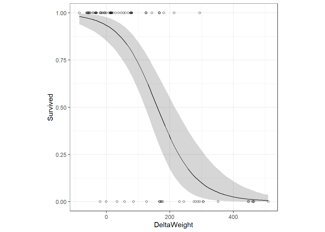
図9.7: Fitted values of the Bernoulli model applied on the crocodile attack data.
##
## Call:
##    c("inla.core(formula = formula, family = family, contrasts = contrasts,
##    ", " data = data, quantiles = quantiles, E = E, offset = offset, ", "
##    scale = scale, weights = weights, Ntrials = Ntrials, strata = strata,
##    ", " lp.scale = lp.scale, link.covariates = link.covariates, verbose =
##    verbose, ", " lincomb = lincomb, selection = selection, control.compute
##    = control.compute, ", " control.predictor = control.predictor,
##    control.family = control.family, ", " control.inla = control.inla,
##    control.fixed = control.fixed, ", " control.mode = control.mode,
##    control.expert = control.expert, ", " control.hazard = control.hazard,
##    control.lincomb = control.lincomb, ", " control.update =
##    control.update, control.lp.scale = control.lp.scale, ", "
##    control.pardiso = control.pardiso, only.hyperparam = only.hyperparam,
##    ", " inla.call = inla.call, inla.arg = inla.arg, num.threads =
##    num.threads, ", " blas.num.threads = blas.num.threads, keep = keep,
##    working.directory = working.directory, ", " silent = silent, inla.mode
##    = inla.mode, safe = FALSE, debug = debug, ", " .parent.frame =
##    .parent.frame)")
## Time used:
##     Pre = 0.592, Running = 0.113, Post = 0.0354, Total = 0.74
## Fixed effects:
##               mean    sd 0.025quant 0.5quant 0.975quant   mode kld
## (Intercept)  2.760 0.516      1.748    2.760      3.772  2.760   0
## DeltaWeight -0.017 0.003     -0.024   -0.017     -0.010 -0.017   0
##
## Marginal log-Likelihood:  -37.99
##  is computed
## Posterior summaries for the linear predictor and the fitted values are computed
## (Posterior marginals needs also 'control.compute=list(return.marginals.predictor=TRUE)')
9.2.2 10.2.2 Model selection with the marginal likelihood
ここでは、ベイズファクター(Bayes factor)を用いてモデル比較を行う方法を解説する。ここで、2つのモデルがあるとしよう。1つ目は先ほど実行したモデルで、切片と体重差を含むモデル(Model1)、もう1つは切片のみを含むモデル(Model2)である。このとき、ベイズファクターは以下のように定義される。
\[ \begin{aligned} \rm{Bayes} \; \rm{factor} &= \frac{Prob(Model1|D)}{Prob(Model2|D)} \\ &= \frac{Prob(D|Model1)}{Prob(D|Model2)} \times \frac{Model1}{Model2} \end{aligned} \]
周辺尤度\(Prob(D|Model1)\)と\(Prob(D|Model2)\)はそれに対数をとったものがINLAの結果で示されている(それぞれ-37.97と-54.43)。各モデルの事前確率\(Prob(Model1), Prob(Model2)\)は分からないが、何も知識がない状況ではどちらのモデルが正しいかはわからない(五分五分)なので、その比は\(0.5/0.5 = 1\)とする。
このとき、ベイズファクターは以下の値になる。この結果は、モデル1が正しい確率がモデル2が正しい確率よりもはるかに大きいことを示す。すなわち、体重差は生存に大きく影響しているといえる。
\[
\begin{aligned}
\rm{Bayes} \; \rm{factor} &= \frac{Prob(D|Model1)}{Prob(D|Model2)} \times \frac{Model1}{Model2}\\
&= \frac{exp(-37.97)}{exp(-54.43)} \times 1\\
&= 14076257
\end{aligned}
\]
過分散の診断を含むモデル診断も行う必要があるが、ここでは省略する。
9.2.3 Binomial GLM
ここからは、商用のダニ駆除剤がミツバチへのダニの寄生に影響するかを調べたMaggi(unpublished data)のデータを用いる。4種類の駆除剤(Toxic)が異なる濃度(Concentration)で使用された24時間後に死亡したダニの数(Dead_mites)がバッチごとに記録されている。Totalはもともといたダニの数を示す。
mite <- read_delim("data/Drugsmites.txt") %>%
  mutate(fToxic = as.factor(Toxic))

datatable(mite,
          options = list(scrollX = 80),
filter = "top")応答変数をバッチごとに死んだダニの割合(Dead_mites/Total)とする以下のモデルを考える。ただし、\(N_i = Total_i\)である。回帰係数は省略している。
\[
\begin{aligned}
&Deadmites_i \sim Binomial(\pi_i, N_i)\\
&E(Deadmites_i) = \pi_i \times N_i \; and \; var(Deadmites_i) = N_i \times \pi_i \times (1-\pi_i)\\
&logit(\pi_i ) = Intercept + Concentration_i + Toxic_i + Concentration_i \times Toxic_i
\end{aligned}
\]
Rでは以下のように実行する。
m10_9 <- inla(Dead_mites ~ Concentration*fToxic,
              family = "binomial",
              data = mite,
              Ntrials = Total,
              control.compute = list(waic = TRUE,
                                     dic = TRUE),
              control.predictor = list(compute = TRUE))
交互作用がないモデルとどちらが良いか確かめるためDICとWAICを用いたモデル選択を行う。結果、交互作用を含むモデルの方がよいことが分かった。
m10_10 <- inla(Dead_mites ~ Concentration + fToxic,
              family = "binomial",
              data = mite,
              Ntrials = Total,
              control.compute = list(waic = TRUE,
                                     dic = TRUE),
              control.predictor = list(compute = TRUE))

waic.10 <- c(m10_9$waic$waic, m10_10$waic$waic)
dic.10 <- c(m10_9$dic$dic, m10_10$dic$dic)

data.frame(type = c("Full", "- Conc × Toxic"),
           WAIC = waic.10,
           DIC = dic.10) %>%
  column_to_rownames(var = "type")
過分散の診断を含むモデル診断も行う必要があるが、ここでは省略する。
9.3 Gamma GLM
ここでは、イタリアのトスカーナ地方のアメリカザリガニについて調査した Ligas (2008) のデータを用いる。746個体について6つの形態学的特徴が記録されている。ここでは、体重(Weight)と性別(Sex)、体長(CTL)のみに着目する。
cray <- read_delim("data/Procambarus.txt") %>%
  mutate(fSex = as.factor(Sex))

datatable(cray,
          options = list(scrollX = 80),
          filter = "top")
以下のモデルを考える。回帰係数は省略している。
\[
\begin{aligned}
&Weight_i \sim Gamma(\mu_i, \phi)\\
&E(Weight_i) = \mu_i \; and \; var(Weight_i) = \frac{\mu_i^2}{\phi}\\
&log(\mu_i) = Length_i + Sex_i + +ength_i \times Sex_i
\end{aligned}
\]
Rでは以下のように実行する。
m10_11 <- inla(Weight ~ CTL*fSex,
               family = "Gamma",
               control.compute = list(waic = TRUE,
                                      dic = TRUE),
               control.family = list(link = "log",
                                     hyper = list(prec = list(
                                       prior = "loggamma",
                                       param = c(1,0.5)
                                     ))),
data = cray)ガンマ分布のパラメータ\(\phi\)は負の二項分布の\(k\)と同じように機能する9。デフォルトの事前分布としては、\(log(\phi)\)に対してガンマ分布が用いられている。INLAでは\(\phi\)はprecisionパラメータと呼ばれ、モデルの結果に推定値が直接示されている。
モデル選択を行うため、交互作用なしのモデルとフルモデルの比較を行ったところ、交互作用のないモデルの方がDICとWAICが低い値をとることが分かった。
m10_11b <- inla(Weight ~ CTL + fSex,
               family = "Gamma",
               control.compute = list(waic = TRUE,
                                      dic = TRUE),
               control.family = list(link = "log",
                                     hyper = list(prec = list(
                                       prior = "loggamma",
                                       param = c(1,0.5)
                                     ))),
               data = cray)

waic.11 <- c(m10_11$waic$waic, m10_11b$waic$waic)
  dic.11 <- c(m10_11$dic$dic, m10_11b$dic$dic)

data.frame(type = c("Full", "- Conc × Toxic"),
           WAIC = waic.11,
           DIC = dic.11) %>%
  column_to_rownames(var = "type")
過分散の診断を含むモデル診断も行う必要があるが、ここでは省略する。
References
というより、負の二項分布はポワソン分布の期待値\(\lambda\)がガンマ分布から得られているとする混合分布である。↩︎