1 Recognizing statistical dependency
1.1 Pseudoreplication
1.1.1 疑似反復とは
疑似反復(pseudoreplication)とは、応答変数のデータが独立ではないにもかかわらず、統計解析にそのことが考慮されていないことを指す。多くの統計解析は全てのデータが独立であることを仮定しているので、もし疑似反復が生じている状態で分析を行うと正しい結果が得られないことが多い。
疑似反復の典型的な例としては、同じ個体から複数のデータが得られている場合が挙げられる。例えば、ある治療薬の効果を調べる場合、各患者について治療前のデータと治療薬を飲んだ後のデータを収集する。もし100人分データを収集するとすれば200個のデータが集まるが、これらのデータが独立であると考えることはできない。なぜなら、同じ患者のデータはその患者特有の属性など(年齢、性別、あるいは観測できない要因など)によって他の患者のデータよりも類似している可能性が高くなるからである。もし独立であると仮定して分析を行うと、実際よりもデータの標準誤差が小さく推定されてしまい、第一種の過誤を犯しやすくなってしまう。
他にも、例えば10個の植木鉢にそれぞれ5個ずつ種子を植えて、その成長度合いを調べる場合を考えてみよう。このとき、合計50個のデータが得られるが、同じ植木鉢に植えられた種子のデータを独立であると考えることはできない。なぜなら、同じ植木鉢の種子はその植木鉢特有の属性(土中の栄養分、日照度合い、あるいは観測できない要因など)によって、他の植木鉢の種子のデータよりも類似している可能性が高くなるからである。
こうした疑似反復に対処するためのアプローチは、混合モデルと呼ばれるものを適用することである(Zuur et al. 2013)。
1.1.2 時空間的な疑似反復
上記のような疑似反復の他にも、時間的あるいは空間的な疑似反復が生じることがある。例えば、あるニホンザルの群れで発情しているメスの数を毎日記録するとしよう。このとき、時間的に近い日のデータ同士はそうでないデータ同士よりも類似する確率が高い。なぜなら、ある日発情していたメスは、その次の日も発情している可能性が高いからである。
図1.1は実際に宮城県金華山島で収集された発情メス数のデータである。実際に、近い日は類似した値をとることが多いことが分かる。このように、時系列データは互いに独立していないことが多い。こうした時間的な疑似相関を考慮せずに分析を行ってしまう(e.g., 毎日の発情メス数が気温によって変わるかを調べるなど)と、誤った結論を導いてしまいかねない。
daily_data <- read_csv("data/daily_data_2021.csv")

daily_data %>%
  filter(duration >= 300) %>%
  ggplot(aes(x = date))+
  geom_line(aes(y = no_est))+
  scale_x_date(date_breaks = "1 week")+
  scale_y_continuous(breaks = seq(0,16,2))+
  theme_bw(base_size=15)+
  theme(axis.text.x = element_text(angle=30,
                                   hjust=1),
        axis.title.y = element_text(angle = 0,
                                   vjust = 0.5),
        aspect.ratio=0.5,
        legend.position = c(0.2,0.9),
        legend.text = element_text(size=10.5,
                                   family = "Yu Mincho"),
        axis.text = element_text(family = "Times New Roman"))+
  labs(x = "",
       y = "発\n情\nメ\nス\n数")+
  guides(linetype = guide_legend(title=NULL))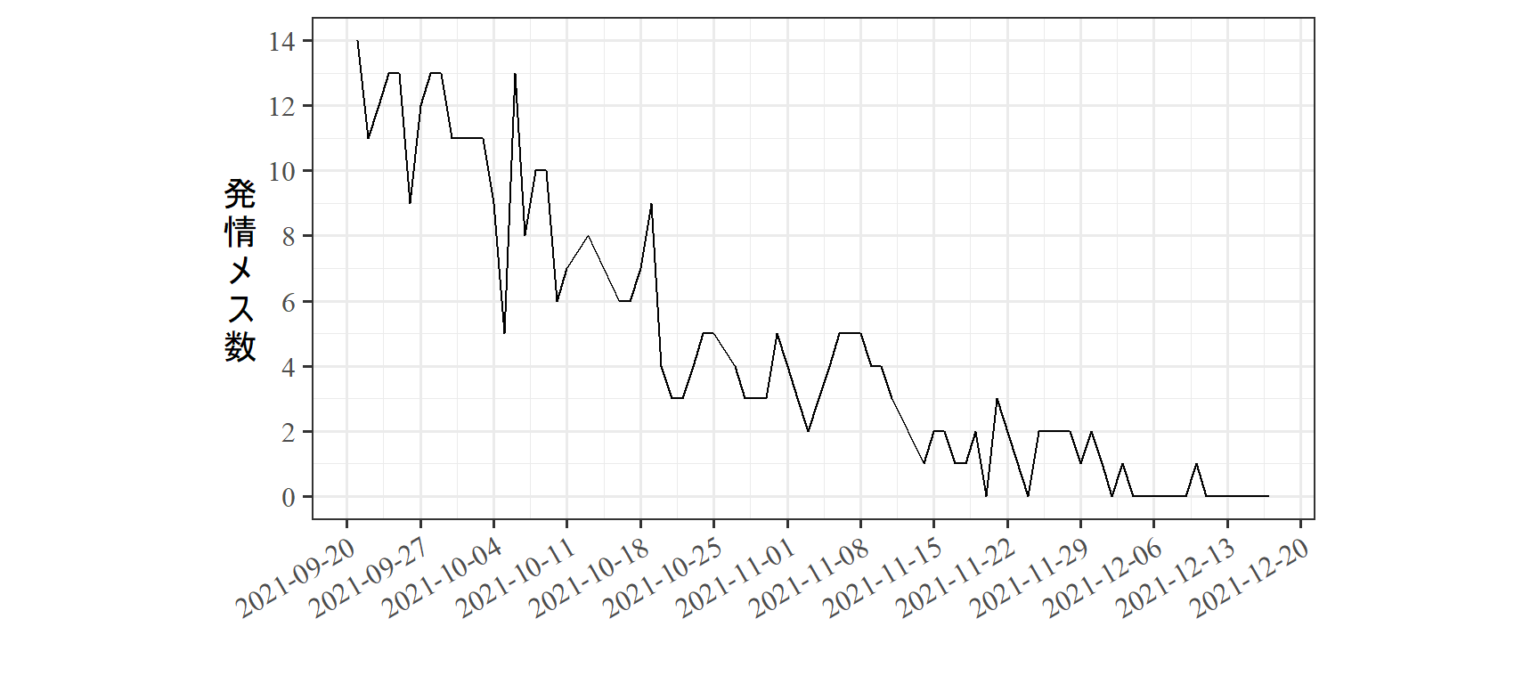
図1.1: 2021年の金華山島B1群における各観察日の発情メス数
地理空間データについても同様のことがいえる。例えば、日本の各都道府県における納豆の消費量について分析するとする(データはこちらから)。このとき、各都道府県のデータを独立と考えることはできない。なぜなら、地理的に近い都道府県は食文化や気候などが類似しており、納豆の消費量も類似している可能性が高くなるからである。
実際、地図上に納豆消費量を図示すると(図1.2)、地理的に近い県は納豆の消費量も類似していることが分かる。このように、空間的データについてもデータ同士に非独立性が生じやすい。
natto <- read_csv("data/natto.csv")
gyuniku <- read_csv("data/gyuniku.csv")
shp <- system.file("shapes/jpn.shp", package = "NipponMap")[1]
pref <- read_sf(shp) %>%
  rename(prefecture = name)

pref %>%
  left_join(gyuniku) %>%
  left_join(natto) -> japan_data

st_crs(japan_data) <- 4326

japan_data %>%
  filter(prefecture != "Okinawa") %>%
  ggplot()+
  geom_sf(aes(fill = natto))+
  theme_bw()+
  theme(aspect.ratio = 1)+
  scale_fill_gradient2(high = muted("blue"), low = muted("red"), mid = "white",
                       midpoint = 3700)+
  labs(fill = "納豆消費量(円)")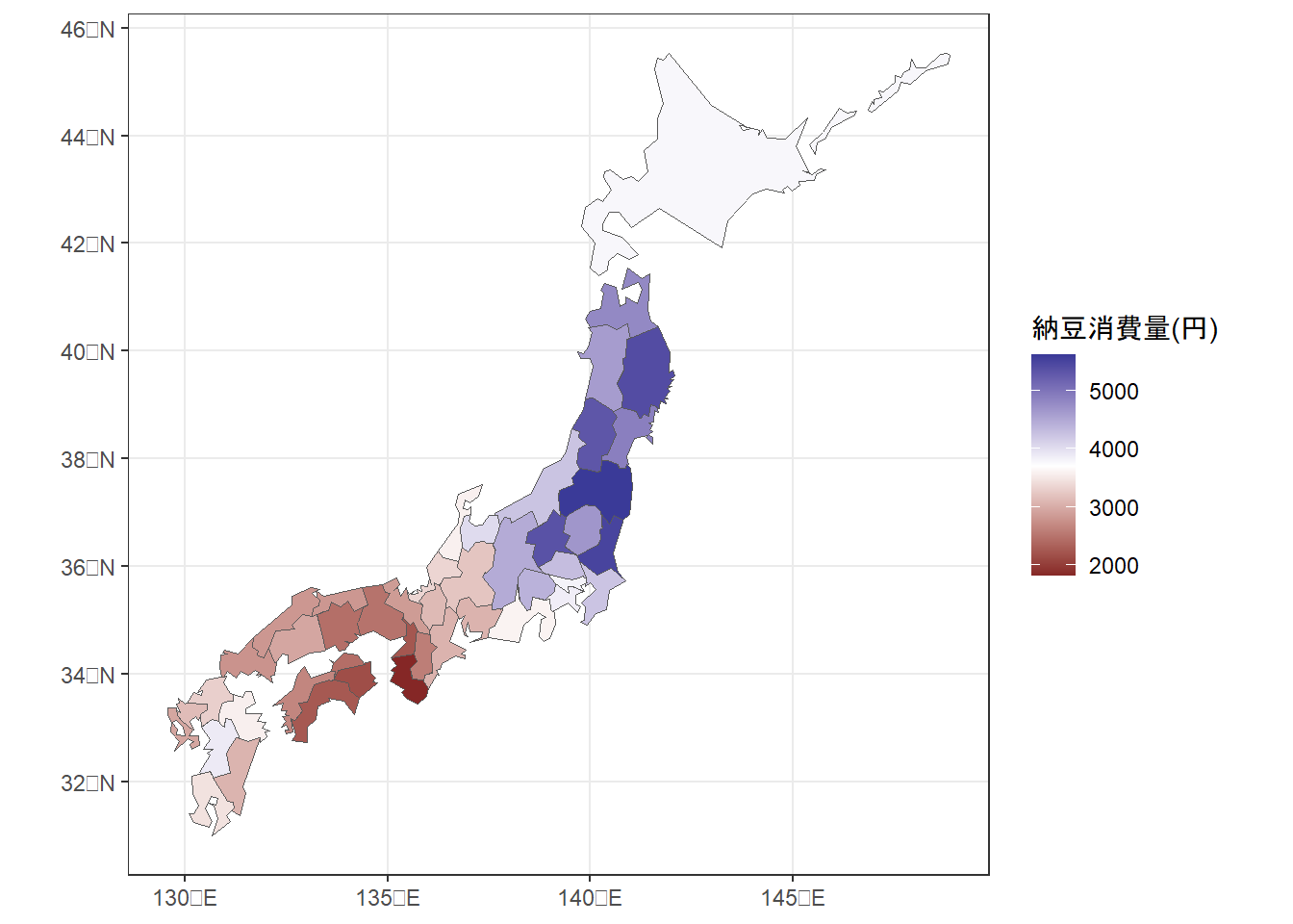
図1.2: 各都道府県の納豆消費量(円)
こうした空間的な疑似反復を考慮せずに分析を行ってしまうと、誤った結論を導いてしまうことになる。例えば、各都道府県の納豆消費量と牛肉消費量が関連しているかを分析するとしよう。図1.3は両者の関連をプロットしたものであるが、プロットだけを見ると両社は強い負の相関を持つように見える(実際、相関係数は-0.737。しかし、先ほど見たように各都道府県のデータは独立ではないので、空間的な非独立性を考慮した分析を行わなければいけない。空間的相関を考慮した分析を行うと、両者の関連はなくなる(こちらを参照)。
japan_data %>%
  ggplot(aes(x = gyuniku, y = natto))+
  geom_point(shape = 1, size = 2)+
  theme_bw()+
  theme(aspect.ratio = 1)+
  labs(y = "納豆消費量(円)", x = "牛肉消費量(g)")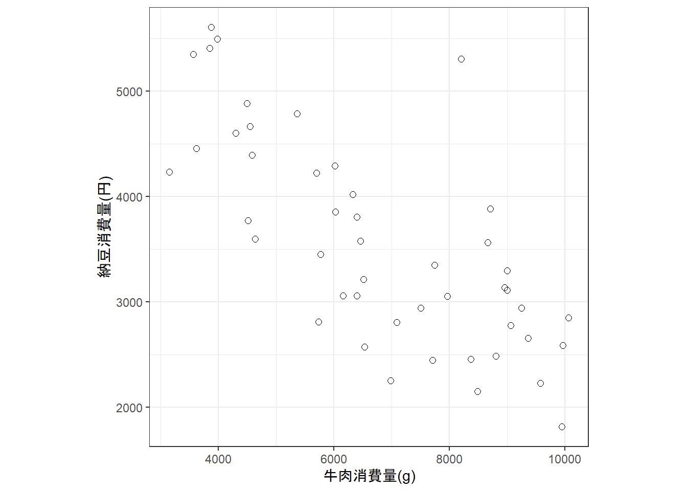
図1.3: 各都道府県の納豆消費量と牛肉消費量
1.2 Linear regression applied to spatial data
本節では、Cruikshanks et al. (2006) のデータを用いる。この研究では、アイルランドの257の川において、川のpHがSDI(Sodium Dominance Index; 陽イオン中のナトリウムイオン)と関連しているかを、緯度(Altitude)やその場所が森林化されているか(Forested)も考慮したうえで調べている。
1.2.1 Visualization
データは以下の通り。
iph <- read_delim("data/Irishph.txt") %>%
  mutate(fForested = ifelse(Forested == "1", "yes", "no")) %>%
  data.frame()

datatable(iph,
          options = list(scrollX = 20),
          filter = "top")
各説明変数との関連は以下の通り。
iph %>%
  dplyr::select(Altitude, pH, fForested, SDI) %>%
  pivot_longer(cols = c(Altitude, SDI)) %>%
  ggplot(aes(x = value, y = pH))+
  geom_point(aes(color = fForested))+
  geom_smooth(aes(color = fForested),
              method = "lm")+
  facet_rep_wrap(~ name,
                 scales = "free_x",
                 repeat.tick.labels = TRUE)+
  theme_bw()+
  theme(aspect.ratio = 1)+
  labs(x = "Covariates")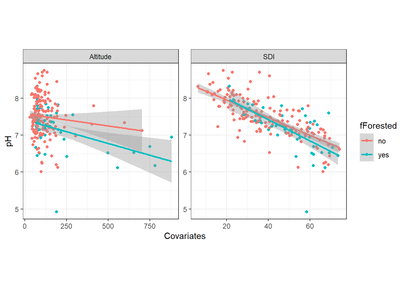
1.2.2 Dependency
以下の線形モデルを適用するとする。
\[ \begin{aligned} pH_i &\sim N(0,\sigma^2)\\ \mu_i &= \beta_1 + \beta_2 \times SDI_i\\ \end{aligned} \]
結果を図示すると以下のようになる。
濃く塗りつぶした部分が95%信頼区間、薄く塗りつぶした部分が95%予測区間である。
ggpredict(m2_1,
          terms = "SDI[7:72,by=0.1]",
          interval = "prediction") %>%
  data.frame() %>%
  mutate(type = "prediction") %>%
  bind_rows(ggpredict(m2_1,
          terms = "SDI[7:72,by=0.1]",
          interval = "confidence") %>%
  data.frame() %>%
    mutate(type = "confidence")) %>%
  rename(SDI = x) %>%
  ggplot(aes(x = SDI, y = predicted))+
  geom_ribbon(aes(ymin = conf.high,
                  ymax = conf.low,
                  fill = type),
              alpha = 0.5)+
  scale_fill_grey()+
  geom_line()+
  geom_point(data = iph,
             aes(y = pH),
             shape = 1)+
  theme_bw()+
  theme(aspect.ratio = 1)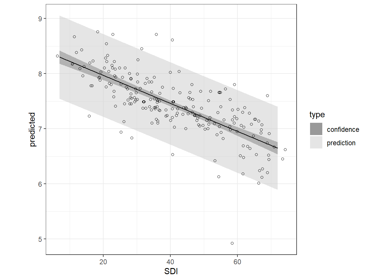
1.2.3 Fit the model
次に、全部の交互作用を含むモデルを考える。
iph %>%
  mutate(logAltitude = log(Altitude,10)) -> iph

m2_2 <- lm(pH ~ SDI*fForested*logAltitude,
           data = iph)
結果は以下の通り。
##
## Call:
## lm(formula = pH ~ SDI * fForested * logAltitude, data = iph)
##
## Residuals:
##      Min       1Q   Median       3Q      Max
## -1.94554 -0.18644 -0.01226  0.21667  1.13820
##
## Coefficients:
##                               Estimate Std. Error t value Pr(>|t|)
## (Intercept)                   8.250624   0.765918  10.772   <2e-16 ***
## SDI                          -0.028011   0.017190  -1.630    0.105
## fForestedyes                  1.794536   2.070682   0.867    0.387
## logAltitude                   0.106199   0.390728   0.272    0.786
## SDI:fForestedyes             -0.008168   0.037112  -0.220    0.826
## SDI:logAltitude               0.001764   0.008614   0.205    0.838
## fForestedyes:logAltitude     -0.885493   1.012152  -0.875    0.383
## SDI:fForestedyes:logAltitude  0.003573   0.017939   0.199    0.842
## ---
## Signif. codes:  0 '***' 0.001 '**' 0.01 '*' 0.05 '.' 0.1 ' ' 1
##
## Residual standard error: 0.3756 on 202 degrees of freedom
## Multiple R-squared:  0.5675, Adjusted R-squared:  0.5525
## F-statistic: 37.86 on 7 and 202 DF,  p-value: < 2.2e-16
あまりに煩雑なのでAICによるモデル選択を行う。
## Start:  AIC=-403.47
## pH ~ SDI * fForested * logAltitude
##
##                             Df Sum of Sq    RSS     AIC
## - SDI:fForested:logAltitude  1 0.0055954 28.498 -405.43
## <none>                                   28.492 -403.47
##
## Step:  AIC=-405.43
## pH ~ SDI + fForested + logAltitude + SDI:fForested + SDI:logAltitude +
##     fForested:logAltitude
##
##                         Df Sum of Sq    RSS     AIC
## - SDI:fForested          1   0.00454 28.503 -407.39
## - SDI:logAltitude        1   0.01654 28.515 -407.31
## <none>                               28.498 -405.43
## - fForested:logAltitude  1   1.01027 29.508 -400.11
##
## Step:  AIC=-407.39
## pH ~ SDI + fForested + logAltitude + SDI:logAltitude + fForested:logAltitude
##
##                         Df Sum of Sq    RSS     AIC
## - SDI:logAltitude        1   0.01443 28.517 -409.29
## <none>                               28.503 -407.39
## - fForested:logAltitude  1   1.08368 29.586 -401.56
##
## Step:  AIC=-409.29
## pH ~ SDI + fForested + logAltitude + fForested:logAltitude
##
##                         Df Sum of Sq    RSS     AIC
## <none>                               28.517 -409.29
## - fForested:logAltitude  1    1.2837 29.801 -402.04
## - SDI                    1   29.3674 57.884 -262.62
##
## Call:
## lm(formula = pH ~ SDI + fForested + logAltitude + fForested:logAltitude,
## data = iph)
##
## Coefficients:
## (Intercept) SDI fForestedyes
## 8.10382 -0.02461 1.29402
## logAltitude fForestedyes:logAltitude
## 0.18292 -0.65962AICが最小のモデルは以下の通り。
1.2.4 Model validation
1.2.4.1 Check homogeinity and model misfit
モデル診断を行う。標準化残差と予測値、各共変量の関係は特にパターンが見られず、問題ないよう。
resid <- rstandard(m2_3)

data.frame(resid = resid,
           fitted = predict(m2_3)) %>%
  ggplot(aes(x = fitted, y = resid))+
  geom_point(shape = 1)+
  theme_bw()+
  theme(aspect.ratio = 1)+
  geom_hline(yintercept = 0,
linetype = "dashed") 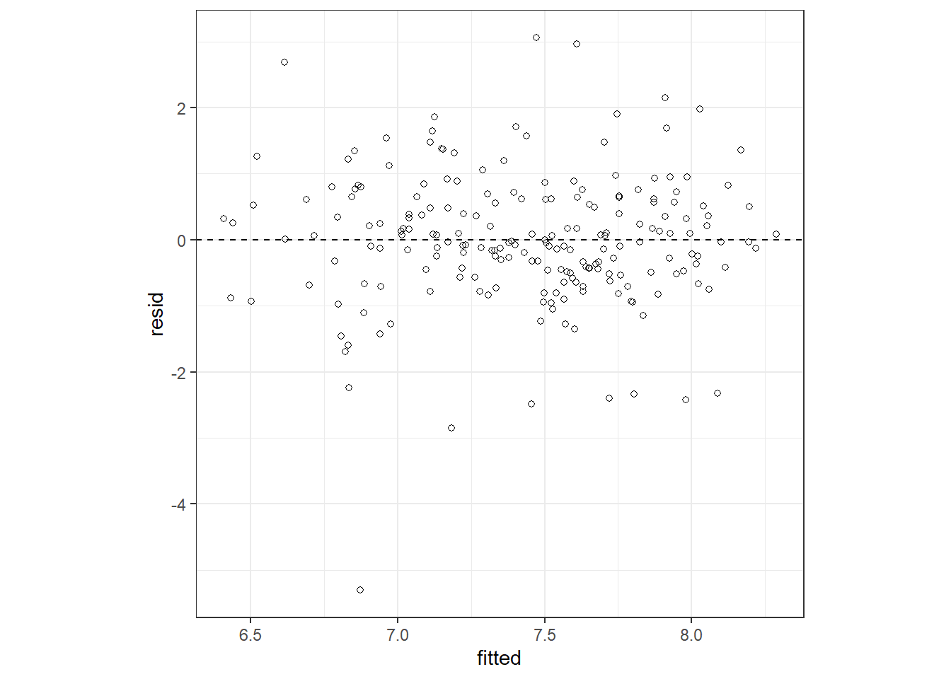
iph %>%
  mutate(resid = resid) %>%
  select(resid, SDI,  logAltitude) %>%
  pivot_longer(cols = c(SDI, logAltitude)) %>%
  ggplot(aes(x = value, y = resid))+
  geom_point(shape = 1)+
  geom_hline(yintercept = 0,
             linetype = "dashed")+
  theme_bw()+
  theme(aspect.ratio = 1)+
  facet_rep_wrap(~ name,
                 repeat.tick.labels = TRUE,
                 scales = "free")+
  theme_bw()+
labs(x = "") 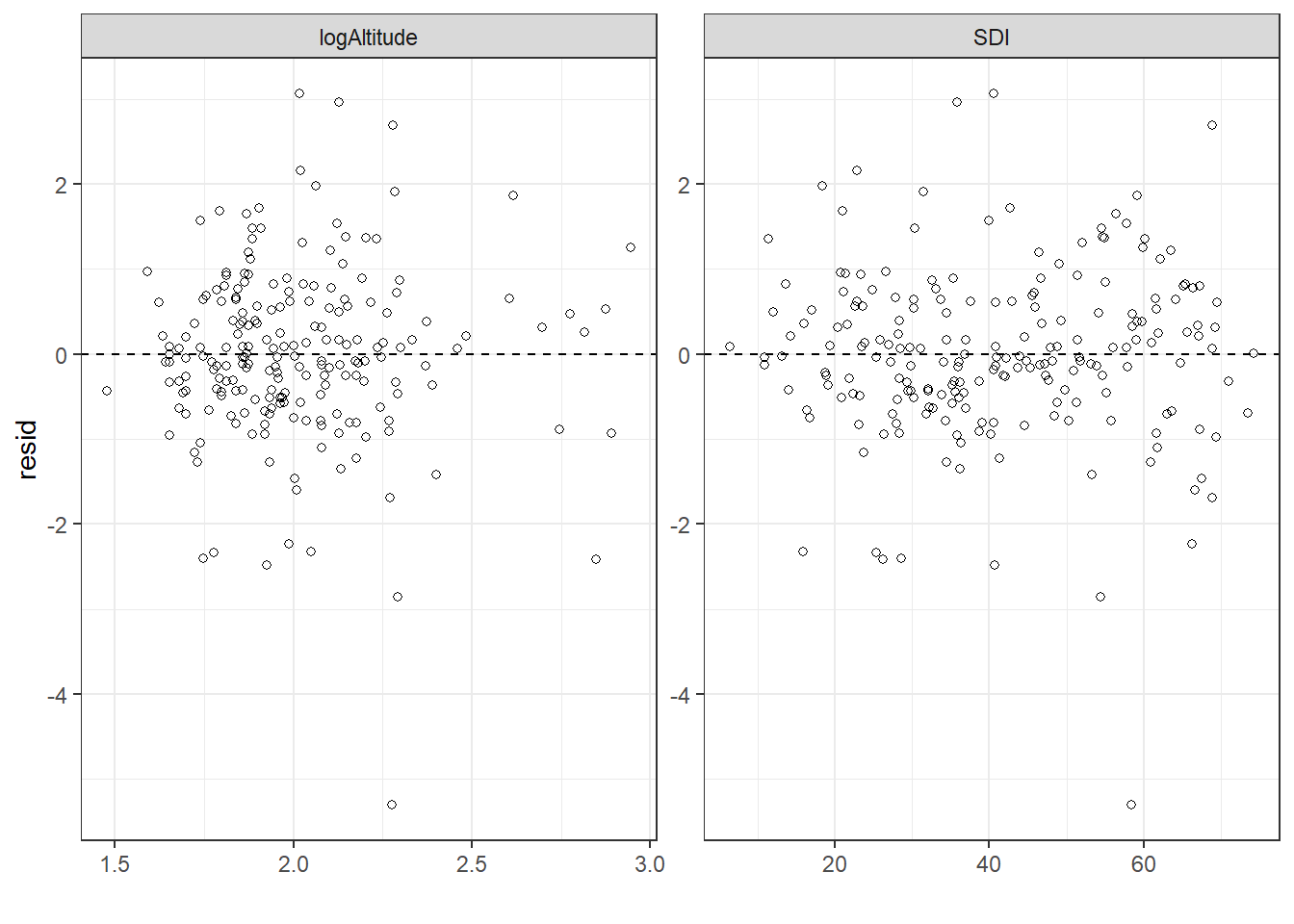
iph %>%
  mutate(resid = resid) %>%
  select(resid, fForested) %>%
  ggplot(aes(x = fForested, y = resid))+
  geom_boxplot()+
  theme_bw()+
  theme(aspect.ratio = 1)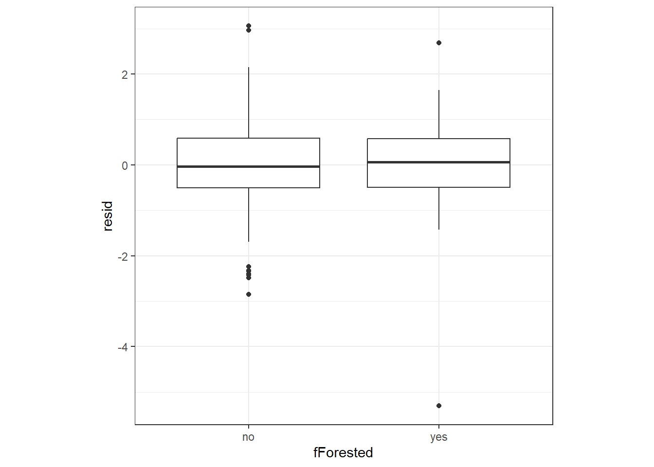
1.2.5 Check spatial dependence
地理的空間上に残差を図示してもパターンがあるかはわかりにくい。
iph %>%
  mutate(resid = resid) %>%
  ggplot(aes(x = Easting, y = Northing))+
  geom_point(shape = 21,
             aes(fill = resid >= 0,
                 size = abs(resid)))+
  scale_fill_manual(values = c("white","black"))+
  theme_bw()+
  theme(aspect.ratio = 1)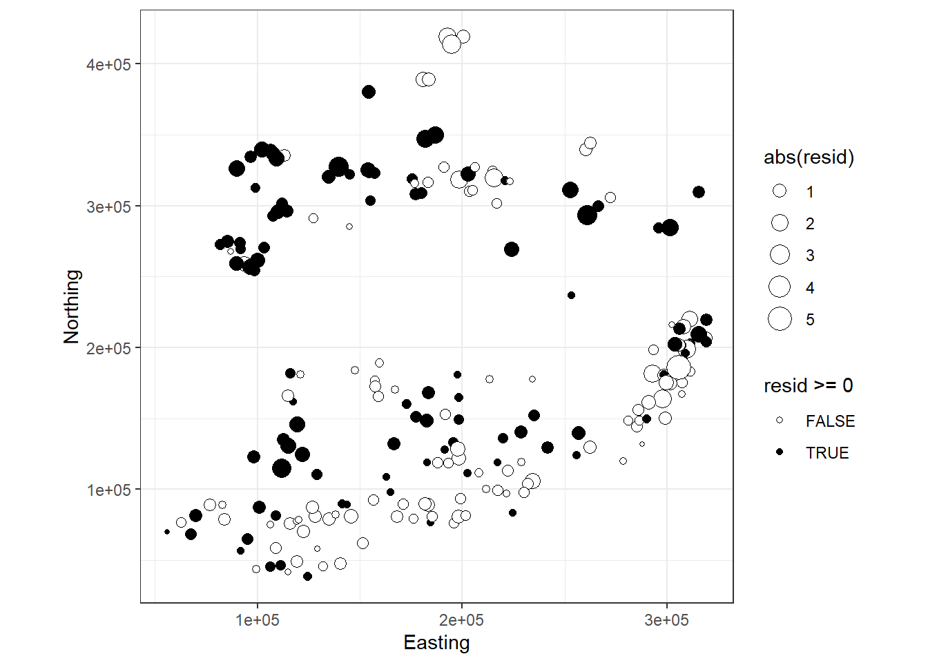
図1.4: Residuals plotted versus spatial position. The width of a point is proportional to the (absolute) value of a residual. Filled circles are positive residuals and open circles are negative residuals. It would be useful to add the contour lines of the Irish borders.
そこで、バリオグラムを作成する。
バリオグラムではまず、データ間の距離がある特定の範囲内にあるデータのペアを抽出する。例えば、図1.5は10kmずつに区切った範囲内にある2つのデータをつないだものである。そのうえで、ある距離範囲カテゴリ(e.g., 10km < dist < 20km)において各データペアの残差の差の二乗を平均したものを算出する。これを全距離範囲カテゴリについて行い、それを図示したものをバリオグラムという。なお、各範囲カテゴリには、少なくとも100ペアくらいはあった方がよい。
crossing(ID1 = iph$ID,
         ID2 = iph$ID) %>%
  left_join(iph %>% select(ID,Easting, Northing),
            by = c("ID1" = "ID")) %>%
  rename(Easting1 = Easting,
         Northing1 = Northing) %>%
  left_join(iph %>% select(ID,Easting, Northing),
            by = c("ID2" = "ID")) %>%
  rename(Easting2 = Easting,
         Northing2 = Northing) %>%
  filter(ID1 != ID2) %>%
  mutate(dist = sqrt((Easting1 - Easting2)^2 + (Northing1 - Northing2)^2)/1000) %>%
  mutate(cat = ifelse(dist < 10, "Distances < 10 km",
                      ifelse(dist < 20, "10 km < Distances < 20 km",
                             ifelse(dist < 30, "20 km < Distances < 30 km",
                                    ifelse(dist < 40, "30 km < Distances < 40 km", "NA"))))) %>%
  mutate(cat2 = ifelse(dist < 40, 1,
                       ifelse(dist < 30, 2,
                              ifelse(dist < 20, 3,
                                     ifelse(dist < 10, 4, "NA"))))) %>%
  filter(cat != "NA") %>%
  mutate(cat = fct_relevel(cat, "Distances < 10 km")) %>%
  ggplot()+
  geom_segment(aes(x = Easting1, xend = Easting2, y = Northing1, yend = Northing2),
               data = . %>% filter(cat2 == "1"))+
  geom_segment(aes(x = Easting1, xend = Easting2, y = Northing1, yend = Northing2),
               data = . %>% filter(cat2 == "2"))+
  geom_segment(aes(x = Easting1, xend = Easting2, y = Northing1, yend = Northing2),
               data = . %>% filter(cat2 == "3"))+
  geom_segment(aes(x = Easting1, xend = Easting2, y = Northing1, yend = Northing2),
               data = . %>% filter(cat2 == "4"))+
  facet_rep_wrap(~cat,
                 repeat.tick.labels = TRUE)+
  theme_bw()+
  theme(aspect.ratio = 1)+
  labs(x = "Easting", y = "Northing")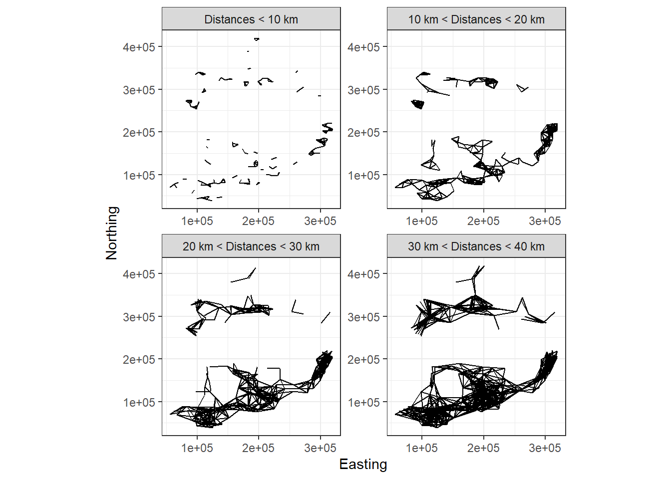
図1.5: Each panel shows c ombinations of any two sampling locations with distances of certain threshold values.
もしデータに空間的な相関がないのであれば、距離の範囲カテゴリに関わらずデータペアの残差の差の平均は一定になるはずである(= バリオグラムはx軸と平行になる)。一方で、例えば空間的に近いデータほど似た残差をとるのであれば、近い距離範囲カテゴリではデータペアの残差の差の平均が小さくなる。
Rでは以下のように実行できる。cressie = TRUEとすることで推定がより頑強になり、外れ値の影響を小さくすることができる。npは各距離範囲カテゴリのデータ数を、distはそれぞれの距離カテゴリーにおけるデータ間の平均距離、gammaは計算されたバリオグラムの値を表す。明らかにプロットは一定の値をとっておらず、強い空間相関があることが予想される(図1.6)。
vario_2_3 <- data.frame(resid = rstandard(m2_3),
                        Easting.km = iph$Easting/1000,
                        Northing.km = iph$Northing/1000)

sp::coordinates(vario_2_3) <- c("Easting.km", "Northing.km")

vario_2_3 %>%
  variogram(resid ~ 1, data = .,
            cressie = TRUE,
            ## 距離が150km以下のデータのみ使用
            cutoff = 150,
            ## 各距離範囲カテゴリの範囲
            width = 10) %>%
  ggplot(aes(x = dist, y = gamma))+
  geom_point(aes(size = np))+
  theme_bw()+
  theme(aspect.ratio = 1)+
  labs(y = "semivariogram")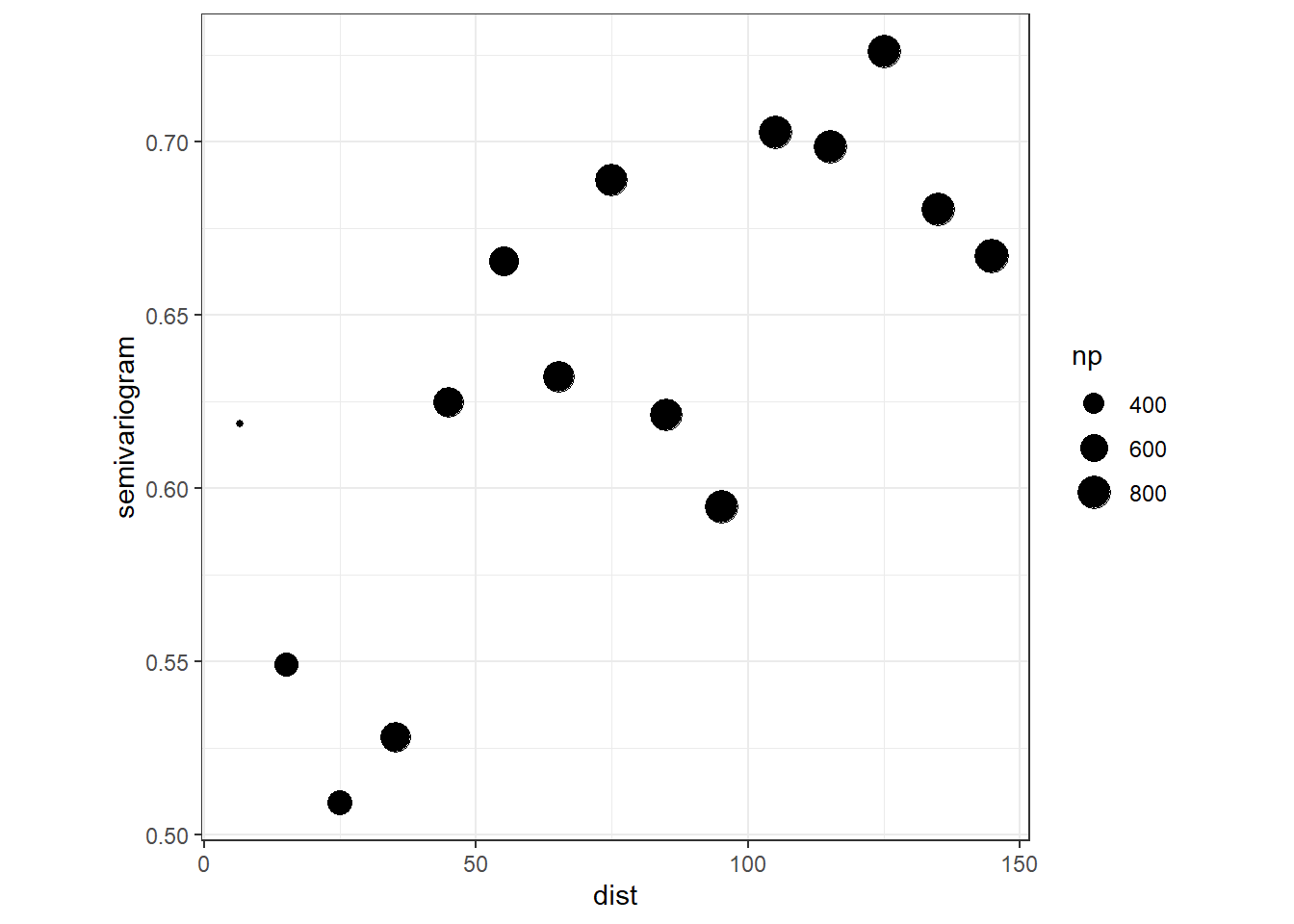
図1.6: m2_3のバリオグラム
南北方向と東西方向の距離を分けて調べることもできる。特に東西方向では明確にバリオグラムが水平ではなく、空間的な独立性がないことが分かる。
vario_2_3 %>%
  variogram(resid ~ Easting.km + Northing.km, data = .,
            ## 0が南北方向、90が東西方向
            alpha = c(0, 90),
            cressie = TRUE,
            cutoff = 150,
            width = 10) %>%
  ggplot(aes(x = dist, y = gamma))+
  geom_point(aes(size = np))+
  theme_bw()+
  theme(aspect.ratio = 1)+
  facet_rep_wrap(~ dir.hor,
                 labeller = as_labeller(c("0" = "North-South",
                                          "90" = "East-West")))+
  labs(y = "semivariogram")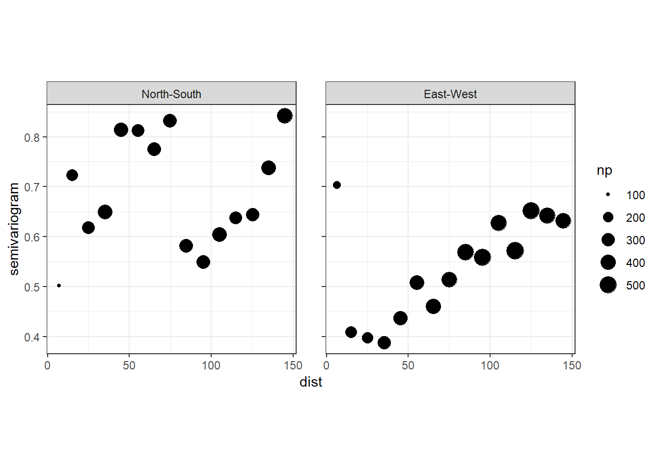
1.3 GAM applied to temporal data
1.3.1 Subnivium temperature data
本節では、 Petty et al. (2015) のデータを用いる。この論文では雪下と地面の間の環境(subnivium)の温度を調べている。積雪量が温度に与える影響を、米ウィスコンシン州の3か所の3つの異なる環境(tall grass prailies, deciduous, coniferous)で検討している。
2013年12月から2014年3月における、日ごとの平均温度が記録されている。各環境に4つずつデータロガーが置かれている。そのため、\(3 \times 4 = 12\)個の時系列データがある。
sn <- read_csv("data/Snow.csv") %>%
  mutate(date = as_datetime(str_c(Year,Month, Day, sep = "-"))) %>%
  mutate(date_num = as.numeric((date - min(date))/(3600*24)) + 1)

datatable(sn,
          options = list(scrollX = 20),
filter = "top")論文に倣い、2013年12月5日から2014年3月3日までのデータを用いる(4 <= date_num <= 92)。
各環境における温度の変化は以下の通り。
sn2 %>%
  ggplot(aes(x = date_num, y = Temp))+
  geom_line(aes(linetype = Logger))+
  facet_rep_wrap(~Type)+
  theme_bw()+
  theme(aspect.ratio = 1.2)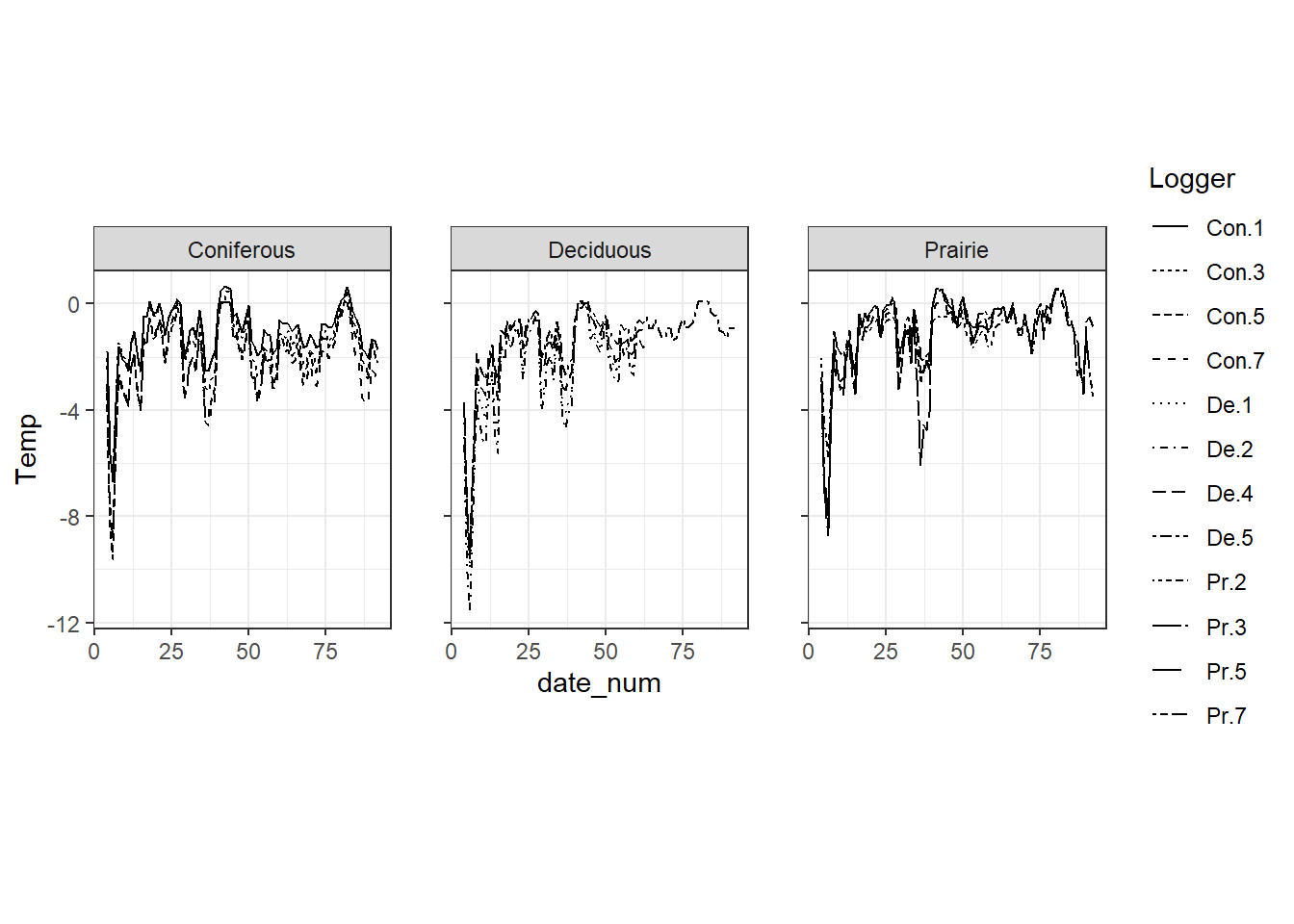
1.3.2 Sources of dependency
同じ環境のロガーはそれぞれ10mしか離れていないので、同じ日におけるこれらのロガーのデータは独立ではない。また、同じロガーのデータについても、時間的な相関があると考えられる(t-1日目の温度とt日目の温度が独立とは考えにくい)。各環境間は距離が離れているので、独立性があると仮定してよさそう。
以下では、こうした非独立性を考慮せずに分析をした場合にどのような問題がが生じるかを見ていく。
1.3.3 The model
以下のGAMMを適用する(回帰係数は省略している)。ロガーIDをランダム切片として入れている。環境ごとにsmootherを推定する。\(t\)は経過日数(date_num)、\(i\)はロガーのidを表す。
\[ \begin{aligned} T_{it} &\sim N(\mu_t, \sigma^2)\\ \mu_{it} &= \alpha + f_j(date\_num_t) + Type_i + a_i\\ a_i &\sim N(0, \sigma_{Logger}^2) \end{aligned} (\#eq:m2.4) \]
Rでは以下のように実行する。
m2_4 <- gamm(Temp ~ s(date_num, by = Type) + Type,
             random = list(Logger =~ 1),
             data = sn2 %>% mutate(Type = as.factor(Type)))
結果は以下の通り。
##
## Family: gaussian
## Link function: identity
##
## Formula:
## Temp ~ s(date_num, by = Type) + Type
##
## Parametric coefficients:
##               Estimate Std. Error t value Pr(>|t|)
## (Intercept)    -1.7363     0.1796  -9.670   <2e-16 ***
## TypeDeciduous  -0.1378     0.2574  -0.535   0.5927
## TypePrairie     0.5000     0.2551   1.960   0.0503 .
## ---
## Signif. codes:  0 '***' 0.001 '**' 0.01 '*' 0.05 '.' 0.1 ' ' 1
##
## Approximate significance of smooth terms:
##                              edf Ref.df     F p-value
## s(date_num):TypeConiferous 8.658  8.658 36.21  <2e-16 ***
## s(date_num):TypeDeciduous  8.205  8.205 62.67  <2e-16 ***
## s(date_num):TypePrairie    8.229  8.229 37.69  <2e-16 ***
## ---
## Signif. codes:  0 '***' 0.001 '**' 0.01 '*' 0.05 '.' 0.1 ' ' 1
##
## R-sq.(adj) =  0.548
## Scale est. = 1.0144 n = 921## Linear mixed-effects model fit by maximum likelihood
## Data: strip.offset(mf)
## AIC BIC logLik
## 2787.212 2840.292 -1382.606
##
## Random effects:
## Formula: ~Xr - 1 | g
## Structure: pdIdnot
## Xr1 Xr2 Xr3 Xr4 Xr5 Xr6 Xr7 Xr8
## StdDev: 20.28316 20.28316 20.28316 20.28316 20.28316 20.28316 20.28316 20.28316
##
## Formula: ~Xr.0 - 1 | g.0 %in% g
## Structure: pdIdnot
## Xr.01 Xr.02 Xr.03 Xr.04 Xr.05 Xr.06 Xr.07 Xr.08
## StdDev: 16.03337 16.03337 16.03337 16.03337 16.03337 16.03337 16.03337 16.03337
##
## Formula: ~Xr.1 - 1 | g.1 %in% g.0 %in% g
## Structure: pdIdnot
## Xr.11 Xr.12 Xr.13 Xr.14 Xr.15 Xr.16 Xr.17 Xr.18
## StdDev: 14.19846 14.19846 14.19846 14.19846 14.19846 14.19846 14.19846 14.19846
##
## Formula: ~1 | Logger %in% g.1 %in% g.0 %in% g
## (Intercept) Residual
## StdDev: 0.3414393 1.007198
##
## Fixed effects: y ~ X - 1
## Value Std.Error DF t-value p-value
## X(Intercept) -1.736302 0.1798447 906 -9.654451 0.0000
## XTypeDeciduous -0.137767 0.2578500 9 -0.534292 0.6061
## XTypePrairie 0.499994 0.2555270 9 1.956717 0.0821
## Xs(date_num):TypeConiferousFx1 -1.238174 1.0476349 906 -1.181875 0.2376
## Xs(date_num):TypeDeciduousFx1 3.652453 1.4161295 906 2.579180 0.0101
## Xs(date_num):TypePrairieFx1 0.042635 1.1659387 906 0.036567 0.9708
## Correlation:
## X(Int) XTypDc XTypPr X(_):TC X(_):TD
## XTypeDeciduous -0.697
## XTypePrairie -0.704 0.491
## Xs(date_num):TypeConiferousFx1 -0.001 0.001 0.001
## Xs(date_num):TypeDeciduousFx1 0.000 0.004 0.000 0.000
## Xs(date_num):TypePrairieFx1 0.000 0.000 0.001 0.000 0.000
##
## Standardized Within-Group Residuals:
## Min Q1 Med Q3 Max
## -5.0136973 -0.4288093 0.0765251 0.5515962 3.2003331
##
## Number of Observations: 921
## Number of Groups:
## g g.0 %in% g
## 1 1
## g.1 %in% g.0 %in% g Logger %in% g.1 %in% g.0 %in% g
## 1 121.3.4 Model validation
ロガーごとの標準化残差を時系列的に図示したのが下図である。ここからパターンを読み取るのは難しい。
sn2 %>%
  mutate(resid = resid(m2_4$lme, type = "n")) %>%
  ggplot(aes(x = date_num, y = resid))+
  geom_point()+
  geom_smooth(color = "grey23")+
  facet_rep_wrap(~Logger,
                 scales = "free_y")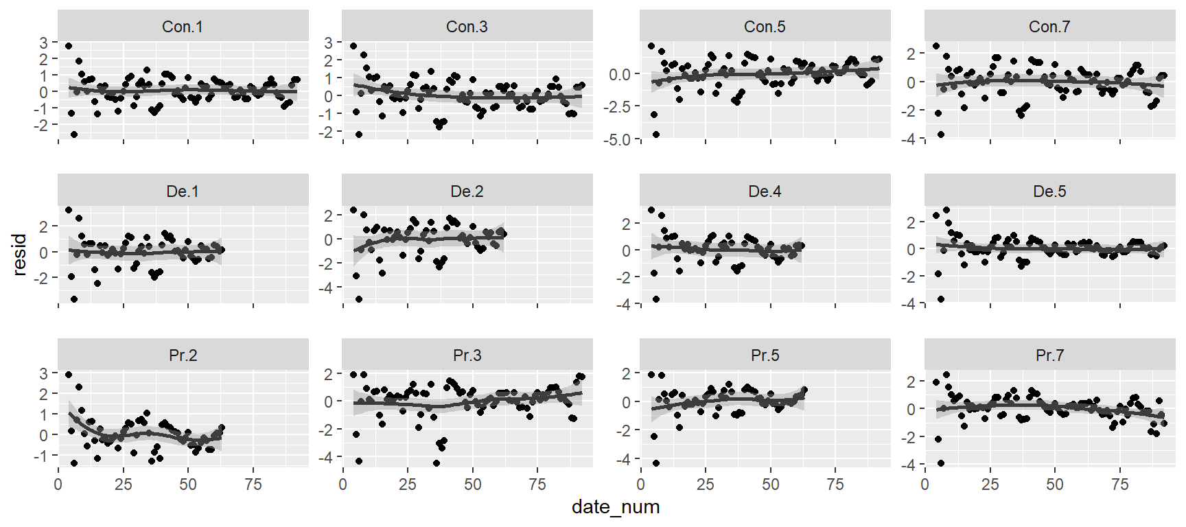
時系列相関があるかを調べるためには、自己相関関数(acf)を描くことが有効である。自己相関関数は、k時点前のデータとの相関をkの関数としてあらわしたものである。
以下で、ロガーごとに時系列相関を算出する。
sn2 %>%
  mutate(resid = resid(m2_4$lme, type = "n")) %>%
  group_by(Logger) %>%
  arrange(date_num, .by_group = TRUE) -> sn3

Loggerid <- unique(sn3$Logger)
all.out <- NULL

for(i in seq_along(Loggerid)){
  data <- sn3 %>% filter(Logger == Loggerid[i])

  ## 各ロガーについて時系列相関を算出
  out.acf <- acf(data$resid,
                 lag.max = 15,
                 plot = FALSE)

  ## 出力をデータフレームに
  out.df <- data.frame(Timelag = out.acf$lag,
                       Acf = out.acf$acf,
                       SE = qnorm(0.975)/sqrt(out.acf$n.used),
                       ID = Loggerid[i])

  ## 全て結合
  all.out <- bind_rows(all.out, out.df)
}
図示したのが下図である。グレーの塗りつぶしは95%信頼区間を表している。図から、全てのロガーにおいて1時点前のデータとの相関が高いことが示唆される。これは、残差に時系列相関があることを示しており、これを考慮したモデルを作成する必要性を示唆している。
all.out %>%
  ggplot(aes(x = Timelag, y = 0))+
  geom_segment(aes(xend = Timelag, yend = Acf))+
  geom_ribbon(aes(ymax = SE, ymin = -SE),
              alpha = 0.3)+
  theme_bw()+
  theme(aspect.ratio = 0.8)+
  facet_rep_wrap(~ID, repeat.tick.labels = TRUE)+
  labs(y = "Auto-correlation")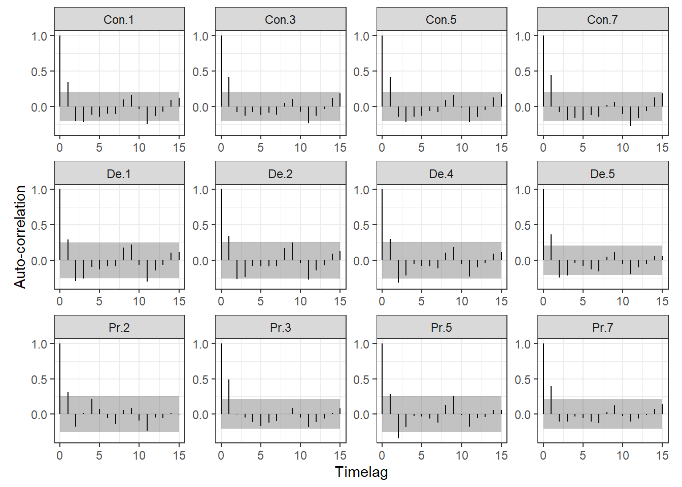
acfの代わりにバリオグラムを用いることもできる。これは、時間間隔が一定でない場合などに有効である。これについては後でもう一度触れる。