11 Linear regression model with spatial dependency for the Irish pH data

本章では、前章で学んだ手法を実際の空間データに適用して分析を行う。

11.1 Introduction

用いるのは第1章で用いた、アイルランドの257の川において、川のpHがSDI(Sodium Dominance Index; 陽イオン中のナトリウムイオン)と関連しているかを、緯度(Altitude)やその場所が森林化されているか(Forested)も考慮したうえで調べた Cruikshanks et al. (2006) のデータである。第1章では、地理的に近いデータほど類似しており、疑似反復の問題を避けるためには空間的相関を考慮したモデルを適用する必要があることを確認した。

11.2 Model formulation

まず、空間的な相関を考慮しないモデルとして以下のモデルを考える。2次の交互作用項と3次の交互作用項をすべて含んでいる。

\[ \begin{aligned} &pH_i \sim N(\mu_i, \sigma^2)\\ &E(pH_i) = \mu_i \; and \; var(pH_i) = \sigma^2\\ &\mu_i = \alpha + \beta_1 \times SDI_i + \beta_2 \times logAltitude_i + \beta_3 + Forested_i \\ & \;\;\;\;\;\;\;\; + \beta_4 \times SDI_i \times LogAltitude_i + \beta_5 \times SDI_i \times Forested_i + \\ & \;\;\;\;\;\;\;\; + \beta_6 \times LogAltitude_i \times Forested_i \\ & \;\;\;\;\;\;\;\; + \beta_7 \times LogAltitude_i \times Forested_i \end{aligned} \]

11.3 Linear regression results

それでは、INLAで上記のモデルを実行する。

iph %>% 
  mutate(logAlt = log10(Altitude)) %>% 
  mutate(fForested = fct_relevel(fForested,"yes","no"))-> iph

m12_1 <- inla(pH ~ logAlt*SDI*fForested,
              family = "gaussian",
              control.predictor = list(compute = TRUE),
              data = iph)

結果は以下の通り。3-way interactionは95%確信区間に0を含んでおり、

m12_1$summary.fixed %>% 
  select(mean, sd, "0.025quant", "0.975quant")

ハイパーパラメータの要約統計量は以下の通り。ここでは、\(\sigma\)について情報を算出した。

tau <- m12_1$marginals.hyperpar$`Precision for the Gaussian observations`
sigma <- inla.tmarginal(function(x) 1/sqrt(x), tau)

sigma_summary <- inla.qmarginal(p = c(0.025, 0.5, 0.975), sigma) %>% data.frame() %>% t()
colnames(sigma_summary) <- c("0.025quant", "0.5quant", "0.975quant")

sigma_summary

##   0.025quant  0.5quant 0.975quant
## .  0.3408095 0.3743001  0.4136209

11.4 Model validation

続いて、モデル診断を行う。

まず、残差と予測値、残差と共変量の関係を調べたら問題はなかった。これは第1と一緒である。

fitted <- m12_1$summary.fitted.values$mean
resid <- iph$pH - fitted

data.frame(fitted = fitted,
           resid = resid) %>% 
  ggplot(aes(x= fitted, y = resid))+
  geom_point(shape = 1)+
  geom_hline(yintercept = 0, linetype = "dashed")+
  theme_bw()+
  theme(aspect.ratio = 1)+
  labs(x= "Fitted values", y = "Residuals") -> p1

data.frame(SDI = iph$SDI,
           resid = resid) %>% 
  ggplot(aes(x= SDI, y = resid))+
  geom_point(shape = 1)+
  geom_hline(yintercept = 0, linetype = "dashed")+
  theme_bw()+
  theme(aspect.ratio = 1)+
  labs(x= "SDI", y = "Residuals") -> p2

data.frame(SDI = iph$logAlt,
           resid = resid) %>% 
  ggplot(aes(x= SDI, y = resid))+
  geom_point(shape = 1)+
  geom_hline(yintercept = 0, linetype = "dashed")+
  theme_bw()+
  theme(aspect.ratio = 1)+
  labs(x= "Log(Altitude)", y = "Residuals") -> p3

data.frame(forested = iph$fForested,
           resid = resid) %>% 
  ggplot(aes(x= forested, y = resid))+
  geom_boxplot()+
  theme_bw()+
  theme(aspect.ratio = 1)+
  labs(x= "Forested", y = "Residuals") -> p4

(p1 + p2)/(p3+p4)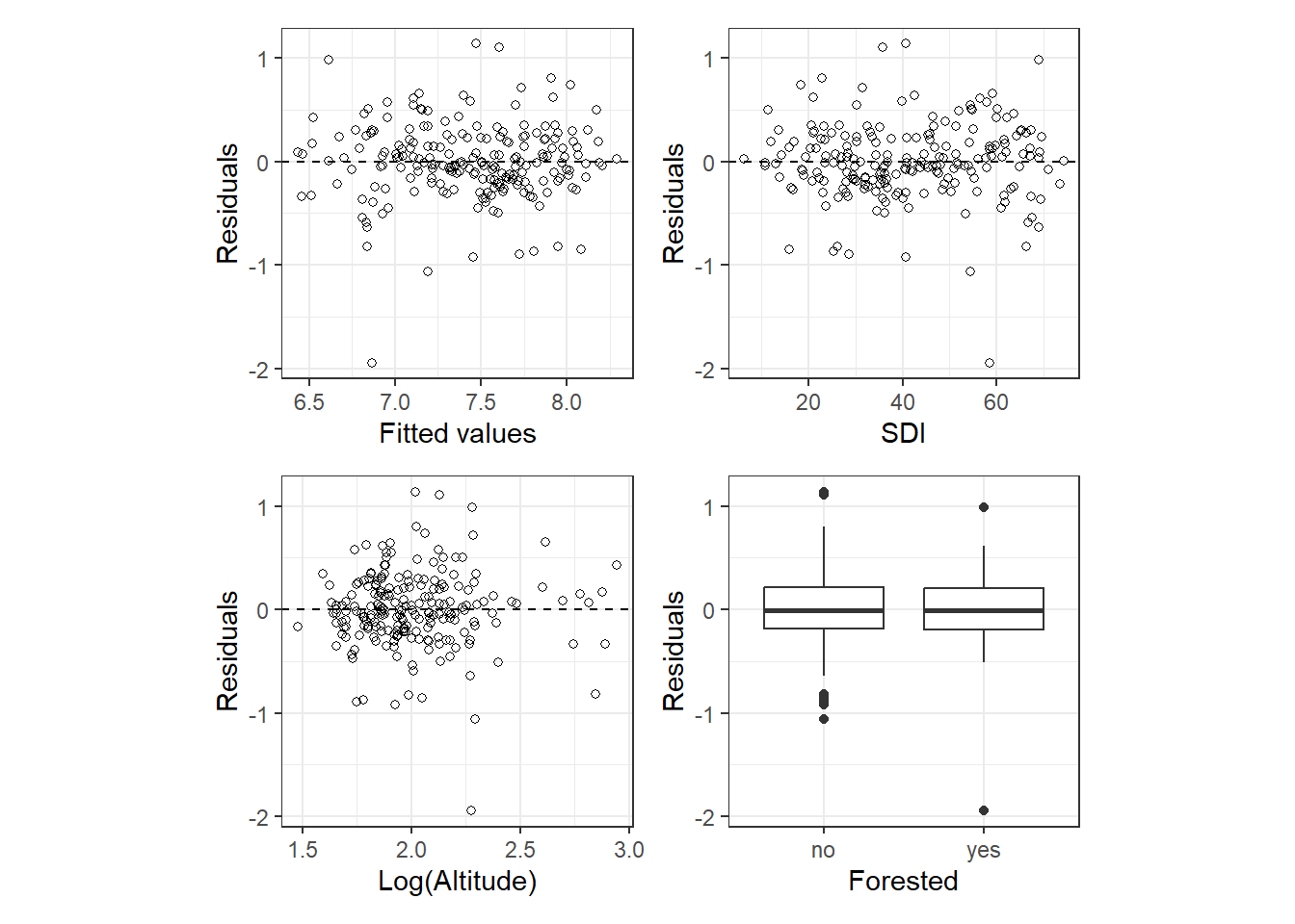

続いて、バリオグラムを確認する。第1章で確認したときと同様、やはり空間的な相関が存在することがわかる。

vario_12_1 <- data.frame(resid = resid,
                        Easting.km = iph$Easting/1000,
                        Northing.km = iph$Northing/1000)

sp::coordinates(vario_12_1) <- c("Easting.km", "Northing.km")

vario_12_1 %>% 
  variogram(resid ~ Easting.km + Northing.km, data = .,
            ## 0が南北方向、90が東西方向
            alpha = c(0, 90),
            cressie = TRUE,
            cutoff = 150,
            width = 10) %>% 
  ggplot(aes(x = dist, y = gamma))+
  geom_point(aes(size = np))+
  theme_bw()+
  theme(aspect.ratio = 1)+
  facet_rep_wrap(~ dir.hor,
                 repeat.tick.labels = TRUE,
                 labeller = as_labeller(c("0" = "North-South",
                                          "90" = "East-West")),
                 scales = "free")+
  labs(y = "semivariogram")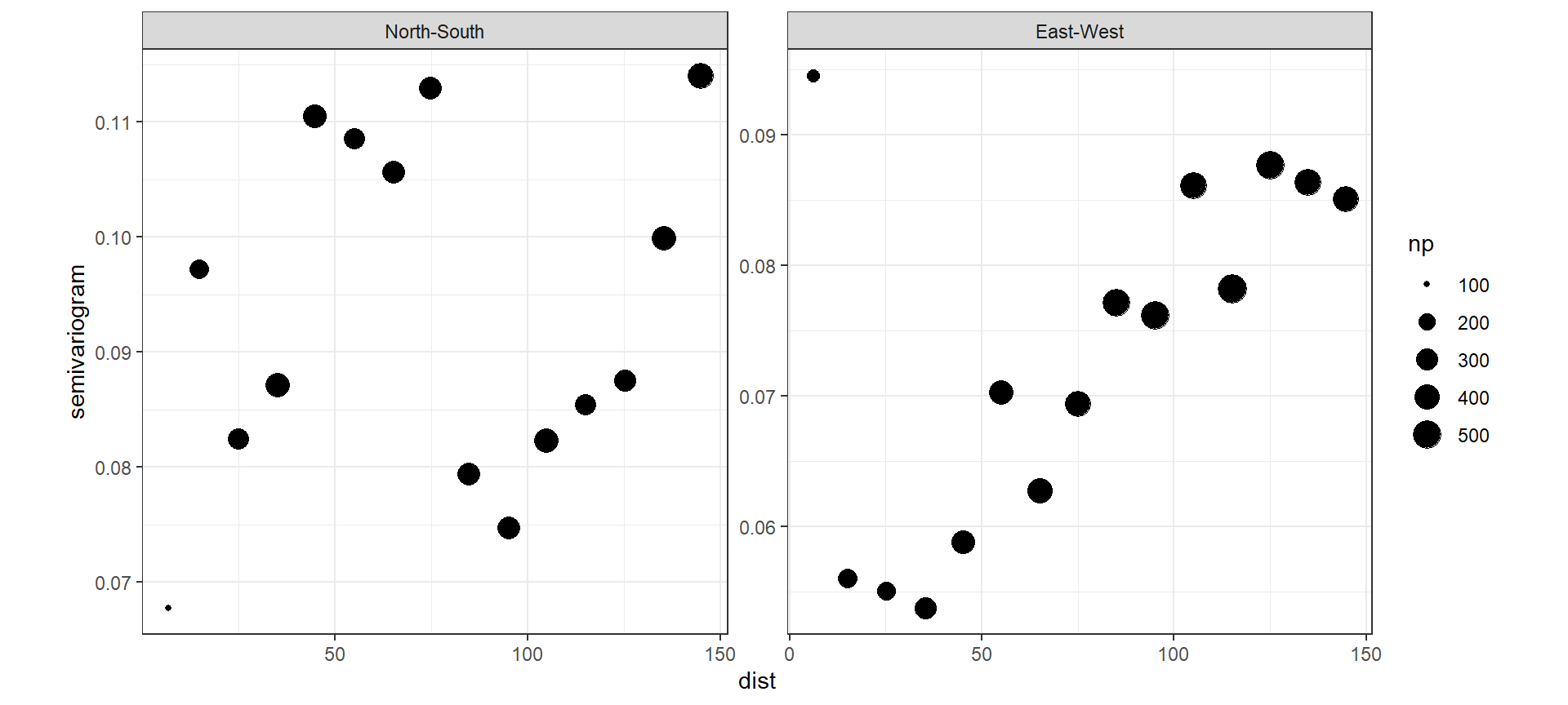

11.5 Adding spatial correlation to the model

それでは、空間的な相関を考慮したモデルを実行する。モデル式は以下の通り。先ほどとの唯一の違いは\(u_i\)が入っている点である。まず、\(u_i\)は正規分布に従っており、ガウス場である。続いて、その分散共分散行列はマルコフ過程に従う(隣り合う観測値のみが相関する)。このとき、\(u_i\)はガウスマルコフランダム場(GMRF)から得られる。\(\bf{\Sigma}\)はMatern関数を用いて表現される。

\[ \begin{aligned} &pH_i \sim N(\mu_i, \sigma^2)\\ &E(pH_i) = \mu_i \; and \; var(pH_i) = \sigma^2\\ &\mu_i = \alpha + \beta_1 \times SDI_i + \beta_2 \times logAltitude_i + \beta_3 + Forested_i \\ & \;\;\;\;\;\;\;\; + \beta_4 \times SDI_i \times LogAltitude_i + \beta_5 \times SDI_i \times Forested_i + \\ & \;\;\;\;\;\;\;\; + \beta_6 \times LogAltitude_i \times Forested_i \\ & \;\;\;\;\;\;\;\; + \beta_7 \times LogAltitude_i \times Forested_i + u_i\\ &u_i \sim GMRF(0,\bf{\Sigma}) \end{aligned} \]

Matern関数のパラメータは、確率偏微分方程式(SPDE)を解くことで求められる。これを解くため、サンプリング空間に多くの三角形から成るメッシュが作られる。最後に、有限要素アプローチ(finite element approach)で各頂点について\(w_k\)が得られ、これをもとに\(u_i\)の事後分布が得られる。

INLAで上記のようなことを行うには、以下のステップを踏む。

1. メッシュを作成する。
   
2. 各頂点の重みづけ因子\(a_{ik}\)を定義する。
   
3. 確率偏微分方程式(SPDE)を定義する。
   
4. ランダム場を定義する。
   
5. メッシュのどの点で応答変数と共変量を得たか、またランダム効果などがあればメッシュのどの点にあるかをINLAに伝える。
   
6. モデル式を決める。
   
7. INLAで空間モデルを実行する。

11.6 Defining the mesh for the Irish pH data

ここでは、アイルランドの河川データに対してメッシュを作成する。まず、データの座標をkmに直す。

iph %>% 
  mutate(Easting.km = Easting/1000,
         Northing.km = Northing/1000) -> iph

2つの場所間の距離\(||s_i - s_j||\)のヒストグラムと、距離の累積割合を示したのが図11.1である。図11.1Bは、50%以上の観測値が200km以内でサンプリングされたことを示している。

dist_iph <- dist(cbind(iph$Easting.km, iph$Northing.km)) %>% as.matrix()
diag(dist_iph) <- NA
dist_iph.vec <- as.vector(dist_iph) %>% na.omit()

data.frame(dist = dist_iph.vec) %>% 
  ggplot(aes(x = dist))+
  geom_histogram(alpha = 0,
                 color = "black",
                 binwidth = 8)+
  theme_bw()+
  theme(aspect.ratio = 1)+
  labs(title = "A", x = "Distances between sites",
       y = "Frequency") -> p1

data.frame(x = sort(dist_iph.vec),
           y = 1:length(dist_iph.vec)/length(dist_iph.vec)) %>% 
  ggplot(aes(x =x, y = y))+
  geom_line()+
  theme_bw()+
  theme(aspect.ratio = 1)+
  labs(title = "B", x = "Distances between sites",
       y = "Cumlutive proportion") -> p2

p1 + p2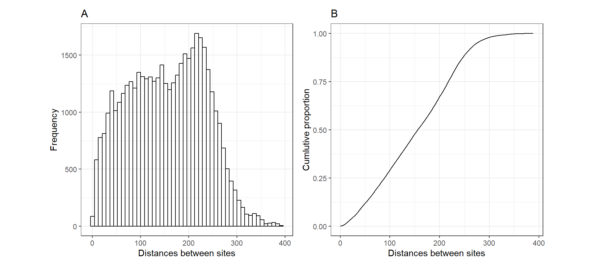

図11.1: A: Histogram of distances between sites in the simulation study. B: Cumulative proportion versus distance between sites.

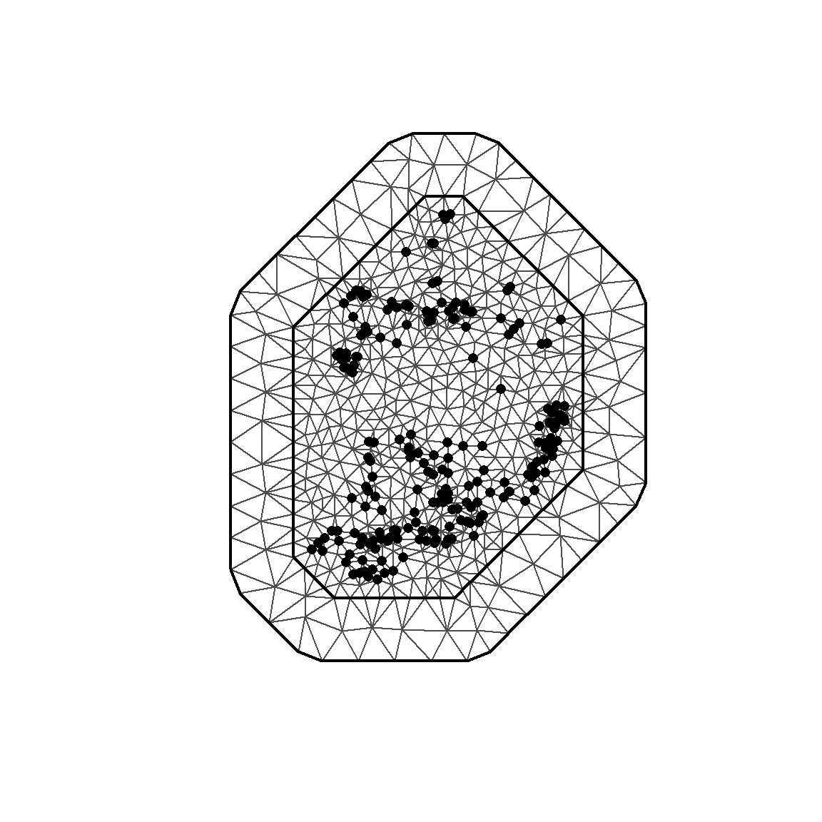
メッシュは以下のように作成する。max.edgeはメッシュの内側と外側の辺の最大の長さをそれぞれ指定する。これが小さいほどメッシュ内の三角形の数は多くなる。作成したメッシュは図11.2の1行目の一番左である。 　　

mesh12_1 <- inla.mesh.2d(loc = cbind(iph$Easting.km, iph$Northing.km),
                         max.edge = c(10,10),
                         cutoff = 0)

メッシュは太い線で内側と外側に分けられている(図11.2)。メッシュは\(w_k\)を計算するのに用いられ、アルゴリズムはその過程で近傍の情報を利用する。もし三角形が調査地の端に位置しているとすると、近傍の三角形が少なくなるので頂点の\(w_k\)のばらつきが大きくなってしまう可能性がある。これを避けるため、メッシュの外側のエリアが使われる。このエリアは2つの太い線に囲われる領域で、サンプリングポイントが存在しない(図11.2)。外側のエリアは内側のエリアに先ほどの問題が生じないようにする緩衝領域だと考えることができる。offsetというオプションを用いると、外側と内側のエリアの範囲を調整することができる。一般的に、外側のエリアはレンジ(空間相関がなくなる距離)よりも広いことが推奨されている。

cutoffオプションは、その距離より近いサンプリングポイント同士が1つの頂点に入れ替えられることを示す。以下、max.edgeとcutoffに様々な値を割り当てたメッシュを作成し、図11.2に示した。

Loc <- cbind(iph$Easting.km, iph$Northing.km)

mesh12_2 <- inla.mesh.2d(loc = Loc,
                         max.edge = c(10,10),
                         cutoff = 10)

mesh12_3 <- inla.mesh.2d(loc = Loc,
                         max.edge = c(50,50))

mesh12_4 <- inla.mesh.2d(loc = Loc,
                         max.edge = c(75,75),
                         cutoff = 1)

mesh12_5 <- inla.mesh.2d(loc = Loc,
                         max.edge = c(25,50),
                         cutoff = 1)

mesh12_6 <- inla.mesh.2d(loc = Loc,
                         max.edge = c(50,80),
                         cutoff = 1)

mesh12_7 <- inla.mesh.2d(loc = Loc,
                         max.edge = c(100,120),
                         cutoff = 1)

mesh12_8 <- inla.mesh.2d(loc = Loc,
                         max.edge = c(150,150),
                         cutoff = 1)

par(mfrow=c(3,3), mar=c(1,1,1,1))

for(i in 1:8){
  plot(get(paste('mesh12_', i, sep = '')), main = "",asp=1)
    points(Loc, col = 2, pch = 16, cex = 1)
}

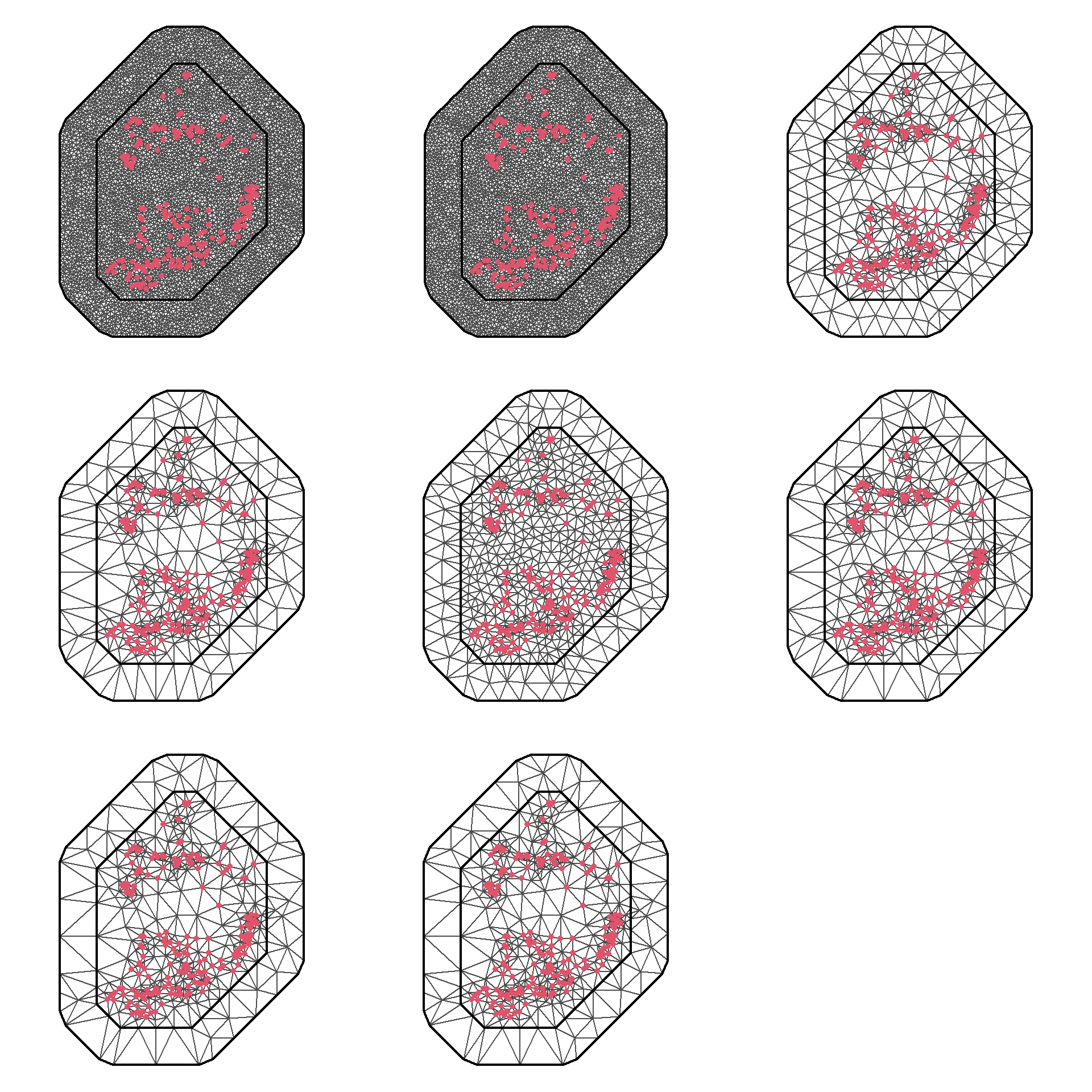
図11.2: Various meshes. Top row from left to right: meshes 1 to 3. Middle row from left to right: meshes 4 to 6. Bottom row from left to right: meshes 7 to 9.

各メッシュの頂点の数は以下の通り。

c(mesh12_1$n, mesh12_2$n, mesh12_3$n, mesh12_4$n, mesh12_5$n, mesh12_6$n, mesh12_7$n, mesh12_8$n)

## [1] 4982 4856  649  523  737  528  515  515

他のアプローチとしては、すべてのサンプリングポイントが境界領域内にあるように境界領域を指定することである。

bound <- inla.nonconvex.hull(Loc)

mesh12_9 <- inla.mesh.2d(loc = Loc,
                         boundary = bound,
                         max.edge = 50,
                         cutoff = 5)

plot(mesh12_9, main = "", asp=1)
points(Loc, col = 2, pch = 16, cex = 1)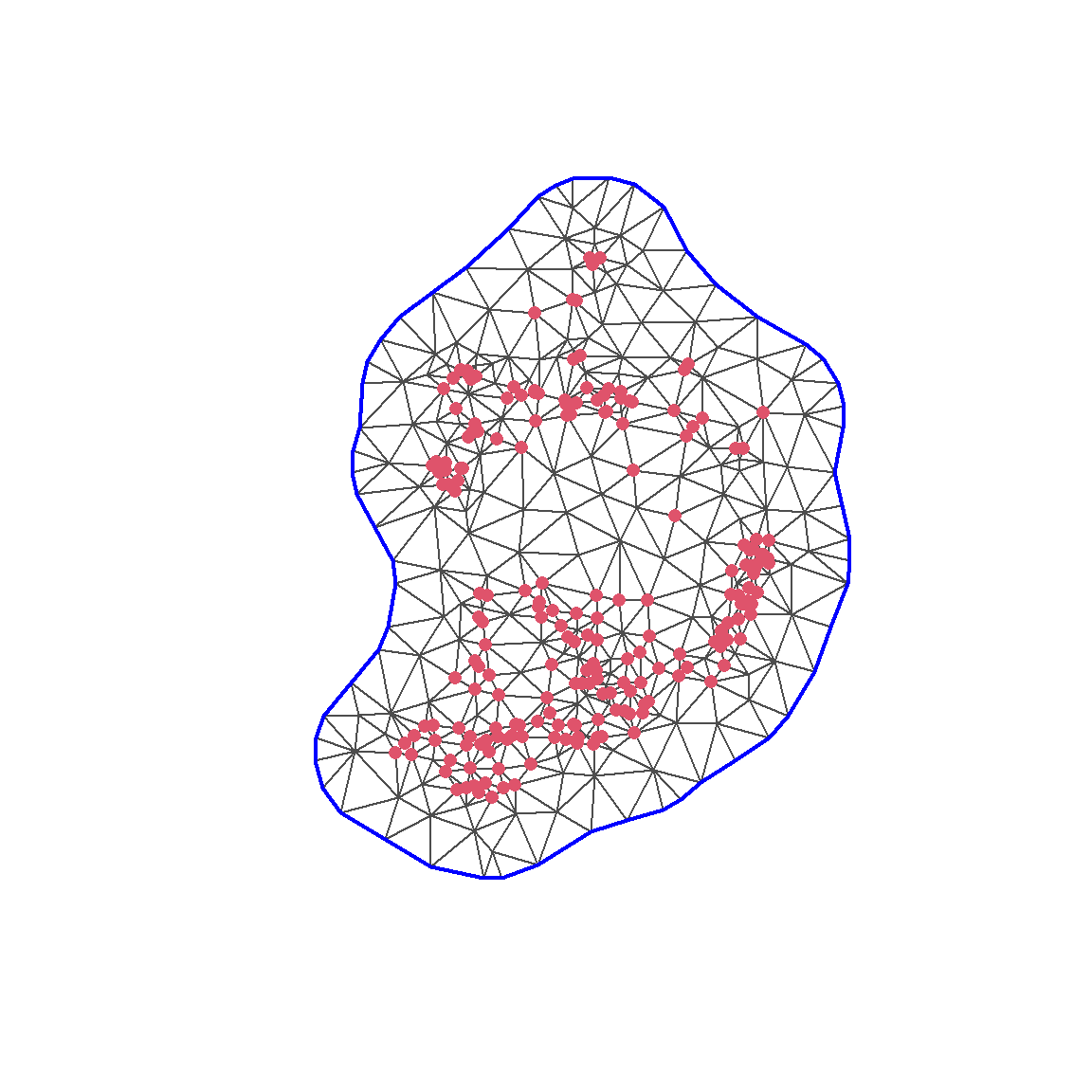

メッシュの選択には、確率偏微分方程式(SPDE)の近似の精度と計算時間のトレードオフがある。700-800の頂点しかない場合は計算が数秒で終わるが、4000-5000個あると数分かかる。一般的にはまず700-800の頂点を持つメッシュで最初の分析を行い、最終的な結果はより多くの頂点を持つメッシュで示す。ひとまず、ここでは737個の頂点があるメッシュmesh12_5を用いて分析する。

plot(mesh12_5, main = "", asp=1)
points(Loc, pch = 16, cex = 1)

11.7 Define the weight factor aik

メッシュmesh12_5は737個の頂点があるので、分析の結果737個の\(w_k\)(\(w_1,w_2,\dots, w_{737}\))の事後分布を得る。また、データは210個あるので、\(u_i\)(\(u_1, u_2, \dots. u_{210}\))も210個ある。メッシュの種類によって各サンプリングポイントはメッシュの三角形内か頂点に配置されるが、今回選択したメッシュ(mesh12_5)では頂点にある。つまり今回の場合は\(s_i\)がk番目の頂点にあるとき、\(u_i\)は\(w_k\)と一致する。一方で、もし\(s_i\)が三角形内にあるのであれば、\(u_i\)はその三角形の頂点\(w_k\)の重みづけ平均になる(第10章、式(10.7)参照)。

\[ u_i = \Sigma_{k=1}^{737} a_{ik} \times w_k \tag{11.1} \]

\(a_{ik}\)は重みづけ関数と呼ばれる。Rでは以下のように確認できる。例えば、\(a_{1k}\)は以下のようになる。

A12_5 <- inla.spde.make.A(mesh12_5, loc = Loc)

A12_5[1,]

##   [1] 0 0 0 0 0 0 0 0 0 0 0 0 0 0 0 0 0 0 0 0 0 0 0 0 0 0 0 0 0 0 0 0 0 0 0 0 0
##  [38] 0 0 0 0 0 0 0 0 0 0 0 0 0 0 0 0 0 0 0 0 0 0 0 0 0 0 0 0 0 0 0 0 1 0 0 0 0
##  [75] 0 0 0 0 0 0 0 0 0 0 0 0 0 0 0 0 0 0 0 0 0 0 0 0 0 0 0 0 0 0 0 0 0 0 0 0 0
## [112] 0 0 0 0 0 0 0 0 0 0 0 0 0 0 0 0 0 0 0 0 0 0 0 0 0 0 0 0 0 0 0 0 0 0 0 0 0
## [149] 0 0 0 0 0 0 0 0 0 0 0 0 0 0 0 0 0 0 0 0 0 0 0 0 0 0 0 0 0 0 0 0 0 0 0 0 0
## [186] 0 0 0 0 0 0 0 0 0 0 0 0 0 0 0 0 0 0 0 0 0 0 0 0 0 0 0 0 0 0 0 0 0 0 0 0 0
## [223] 0 0 0 0 0 0 0 0 0 0 0 0 0 0 0 0 0 0 0 0 0 0 0 0 0 0 0 0 0 0 0 0 0 0 0 0 0
## [260] 0 0 0 0 0 0 0 0 0 0 0 0 0 0 0 0 0 0 0 0 0 0 0 0 0 0 0 0 0 0 0 0 0 0 0 0 0
## [297] 0 0 0 0 0 0 0 0 0 0 0 0 0 0 0 0 0 0 0 0 0 0 0 0 0 0 0 0 0 0 0 0 0 0 0 0 0
## [334] 0 0 0 0 0 0 0 0 0 0 0 0 0 0 0 0 0 0 0 0 0 0 0 0 0 0 0 0 0 0 0 0 0 0 0 0 0
## [371] 0 0 0 0 0 0 0 0 0 0 0 0 0 0 0 0 0 0 0 0 0 0 0 0 0 0 0 0 0 0 0 0 0 0 0 0 0
## [408] 0 0 0 0 0 0 0 0 0 0 0 0 0 0 0 0 0 0 0 0 0 0 0 0 0 0 0 0 0 0 0 0 0 0 0 0 0
## [445] 0 0 0 0 0 0 0 0 0 0 0 0 0 0 0 0 0 0 0 0 0 0 0 0 0 0 0 0 0 0 0 0 0 0 0 0 0
## [482] 0 0 0 0 0 0 0 0 0 0 0 0 0 0 0 0 0 0 0 0 0 0 0 0 0 0 0 0 0 0 0 0 0 0 0 0 0
## [519] 0 0 0 0 0 0 0 0 0 0 0 0 0 0 0 0 0 0 0 0 0 0 0 0 0 0 0 0 0 0 0 0 0 0 0 0 0
## [556] 0 0 0 0 0 0 0 0 0 0 0 0 0 0 0 0 0 0 0 0 0 0 0 0 0 0 0 0 0 0 0 0 0 0 0 0 0
## [593] 0 0 0 0 0 0 0 0 0 0 0 0 0 0 0 0 0 0 0 0 0 0 0 0 0 0 0 0 0 0 0 0 0 0 0 0 0
## [630] 0 0 0 0 0 0 0 0 0 0 0 0 0 0 0 0 0 0 0 0 0 0 0 0 0 0 0 0 0 0 0 0 0 0 0 0 0
## [667] 0 0 0 0 0 0 0 0 0 0 0 0 0 0 0 0 0 0 0 0 0 0 0 0 0 0 0 0 0 0 0 0 0 0 0 0 0
## [704] 0 0 0 0 0 0 0 0 0 0 0 0 0 0 0 0 0 0 0 0 0 0 0 0 0 0 0 0 0 0 0 0 0 0

11.8 Define the SPDE

空間相関を持つランダム切片\(u_i\)で、その分散共分散行列がMatern関数で表現されるとき、SPDEは以下のように定義できる。alpha = 2はMatern関数のパラメータ\(\nu\)が1であることを示す(式(10.6)を参照)。

spde <- inla.spde2.matern(mesh12_5, alpha = 2)

11.9 Define the spatial field

続いて、ランダム切片の行列\(\bf{u}\)を求めるためのリストを作成する。\(\bf{u}\)は\(\bf{A}\)と\(\bf{w}\)を以下のように定義するとき、\(\bf{u} = \bf{A} \times \bf{w}\)と書ける。\(\bf{w}\)はINLAで推定する必要がある。

\[ \begin{aligned} &\bf{A} = \begin{pmatrix} a_{1,1} & a_{1,2} & \cdots & a_{1,737} \\ \vdots & \ddots & & \vdots \\ a_{210,1} & a_{210,2} & \cdots & a_{210,737} \end{pmatrix} \\ &\bf{w} = (w_1, w_2, \dots, w_{737}) \end{aligned} \tag{11.2} \]

\(\bf{w}\)はINLAで推定する必要がある。これは以下のようにできる。w.index中のwは1から737の数字を含む。w.groupとw.replについては時空間モデルを実行するときに解説する。

w.index <- inla.spde.make.index(
  name = 'w',
  n.spde = spde$n.spde,
  n.group = 1,
  n.repl = 1)

str(w.index)

## List of 3
##  $ w      : int [1:737] 1 2 3 4 5 6 7 8 9 10 ...
##  $ w.group: int [1:737] 1 1 1 1 1 1 1 1 1 1 ...
##  $ w.repl : int [1:737] 1 1 1 1 1 1 1 1 1 1 ...

11.10 Define the stack

続いて、メッシュのどの点で応答変数と共変量を得たかをINLAに伝える必要がある。Rでは、inla.stack関数を用いてこれを行う。これについて理解するため、まずモデルをマトリックス形式で書く。

\[ \mu_i = \alpha + \Sigma_{j = 1}^7 \beta_j X_{ij} + u_i \]

\(X_{ij}\)は交互作用項を含む説明変数(\(SDI_i,LogAltitude_i, \dots, SDI_i \times LogAltitude_i \times Forested_i\))を含む。また、式(11.1)よりこの式は以下のように変形できる。

\[ \mu_i = \alpha + \Sigma_{j = 1}^7 \beta_j X_{ij} + \Sigma_{k=1}^{731} a_{ik} \times w_k \]

行列式で書くと以下のように書ける。
\[ \bf{X} = 1 \times \alpha + \bf{X \times \beta} + \bf{A \times w} \tag{11.3} \]

ハイパーパラメータはpHが得られる正規分布の標準偏差\(\sigma\)、Matern関数の\(\kappa\)と\(u_i\)の分散共分散行列の\(\sigma_u\)、そして\(\bf{w}\)である。式(11.3)を実行するためには、INLAにinla.stack関数で3つの要素を与える必要がある。

一つ目は共変量を含む行列\(\bf{X}\)で、以下のように作成する。

Xm <- model.matrix(~ logAlt * SDI * fForested, 
                   data = iph)

X <- data.frame(Alt          = Xm[,2],
                SDI          = Xm[,3],
                fFor         = Xm[,4],
                Alt.SDI      = Xm[,5],
                Alt.fFor     = Xm[,6],
                SDI.fFor     = Xm[,7],
                Alt.SDI.fFor = Xm[,8])

それでは、inla.stack関数でINLAに情報を与える。これで作られたオブジェクトは”stack”といわれる。Aのリストはガウス場への射影行列で、effectsの各要素に対応している。

N <- nrow(iph)

StackFit <- inla.stack(
             tag = "Fit",
             data = list(y = iph$pH),  
               A = list(1, 1, A12_5),                  
               effects = list(   
                  Intercept = rep(1, N),
                  X = X,
                  w = w.index))

11.11 Define the formula for the spatial model

それでは、以下で空間相関のあるモデルとないモデルをフィットする。煩雑になるので、モデル式はあらかじめ作っておく。

## 空間相関なし
f2a <- y ~ -1 + Intercept + Alt  + SDI + fFor + 
           Alt.SDI + Alt.fFor + SDI.fFor + 
           Alt.SDI.fFor

## 空間相関あり
f2b <- y ~ -1 + Intercept + Alt  + SDI + fFor + 
           Alt.SDI + Alt.fFor + SDI.fFor + 
           Alt.SDI.fFor + f(w, model = spde)

11.12 Execute the spatial model in R

それでは、モデルを実行する。

m12_2a <- inla(f2a,
               family = "gaussian",
               data = inla.stack.data(StackFit),
               control.compute = list(dic = TRUE,
                                      waic = TRUE),
               control.predictor = list(A = inla.stack.A(StackFit)))

m12_2b <- inla(f2b,
               family = "gaussian",
               data = inla.stack.data(StackFit),
               control.compute = list(dic = TRUE,
                                      waic = TRUE),
               control.predictor = list(A = inla.stack.A(StackFit)))

DICとWAICを用いてモデル比較を行うと、空間相関を考慮した方がはるかにいいことが分かる。

waic12_2 <- c(m12_2a$waic$waic, m12_2b$waic$waic)
dic12_2 <- c(m12_2a$dic$dic, m12_2b$dic$dic)
modelcomp12_2 <- cbind(waic12_2, dic12_2)
rownames(modelcomp12_2) <- c("Gaussian lm", "Gaussian lm + SPDE")

modelcomp12_2

##                    waic12_2  dic12_2
## Gaussian lm        196.9916 194.5744
## Gaussian lm + SPDE 127.7375 124.2912

11.13 Results

ハイパーパラメータ以外の結果は以下の通り。

m12_2a$summary.fixed[,c("mean","sd","0.025quant","0.975quant")] %>% 
  mutate_if(is.numeric, ~round(.,3)) %>% 
  bind_cols(m12_2b$summary.fixed[,c("mean","sd","0.025quant","0.975quant")] %>% 
              mutate_if(is.numeric, ~round(.,3)) %>% 
              rename(" mean" = 1, " sd" = 2, " 0.025quant" = 3, " 0.975quanr" = 4)) %>% 
  kbl(align = "lcccccccc") %>% 
  add_header_above(c("", "空間相関なし" = 4, "空間相関有り" = 4)) 

	空間相関なし				空間相関有り
	mean	sd	0.025quant	0.975quant	mean	sd	0.025quant	0.975quanr
Intercept	8.247	0.764	6.747	9.748	8.928	0.706	7.541	10.312
Alt	0.108	0.390	-0.658	0.873	-0.245	0.350	-0.932	0.443
SDI	-0.028	0.017	-0.062	0.006	-0.044	0.016	-0.076	-0.012
fFor	1.790	2.062	-2.259	5.839	0.852	1.775	-2.633	4.336
Alt.SDI	0.002	0.009	-0.015	0.019	0.010	0.008	-0.005	0.026
Alt.fFor	-0.883	1.008	-2.862	1.096	-0.335	0.873	-2.048	1.379
SDI.fFor	-0.008	0.037	-0.081	0.064	0.006	0.032	-0.057	0.068
Alt.SDI.fFor	0.004	0.018	-0.032	0.039	-0.005	0.015	-0.035	0.025

事後平均と95%確信区間を図示すると以下のようになる。そこまで大きい違いはないので、空間的相関を表すランダム効果の効果はそこまで大きくないのかもしれない。

m12_2a$summary.fixed[,c("mean","0.025quant","0.975quant")] %>% 
  mutate(model = "m12_2a") %>% 
  rownames_as_column(var = "parameter") %>% 
  bind_rows(m12_2b$summary.fixed[,c("mean","0.025quant","0.975quant")] %>% 
              mutate(model = "m12_2b") %>% 
              rownames_as_column(var = "parameter")) %>% 
  ggplot(aes(x = model, y = mean))+
  geom_errorbar(aes(ymin = `0.025quant`, ymax = `0.975quant`),
                width = 0.2)+
  geom_point()+
  geom_hline(yintercept= 0,
             linetype = "dashed")+
  facet_rep_wrap(~parameter, repeat.tick.labels = TRUE,
                 scales = "free")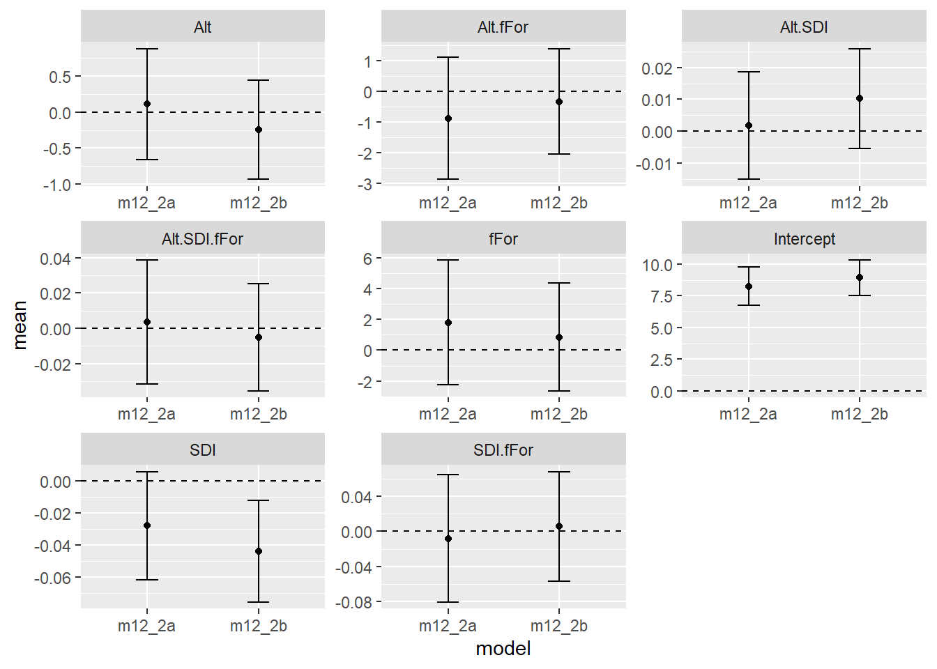

続いて、ハイパーパラメータの結果を見ていく。推定の結果、\(\kappa\)と\(\sigma_u\)の事後平均はそれぞれ0.0319と0.2804であることが分かった。レンジの事後平均は105.61である。

SpFi.w <- inla.spde2.result(inla = m12_2b,
                          name = "w",
                          spde = spde,
                          do.transfer = TRUE)

## Kappa
kappa <- inla.emarginal(function(x) x, SpFi.w$marginals.kappa[[1]])
kappa

## [1] 0.03180548

##sigma
sigma <- inla.emarginal(function(x) sqrt(x), SpFi.w$marginals.variance.nominal[[1]])  
sigma

## [1] 0.2804851

## range  
range = inla.emarginal(function(x) x, SpFi.w$marginals.range.nominal[[1]])
range

## [1] 105.7647

\(\kappa\)が分かればMatern関数を描写することができる。

D <- as.vector(dist(mesh12_5$loc[,1:2]))
d.vec <- seq(0, max(D), length = 100)
corM <- (kappa*d.vec)*besselK(kappa*d.vec,1)
corM[1] <- 1

data.frame(Distance = d.vec,
           Correlation = corM) %>% 
  ggplot(aes(x = Distance, y = Correlation))+
  geom_line()+
  geom_vline(xintercept = range,
             linetype = "dashed")+
  theme_bw()+
  theme(aspect.ratio = 1)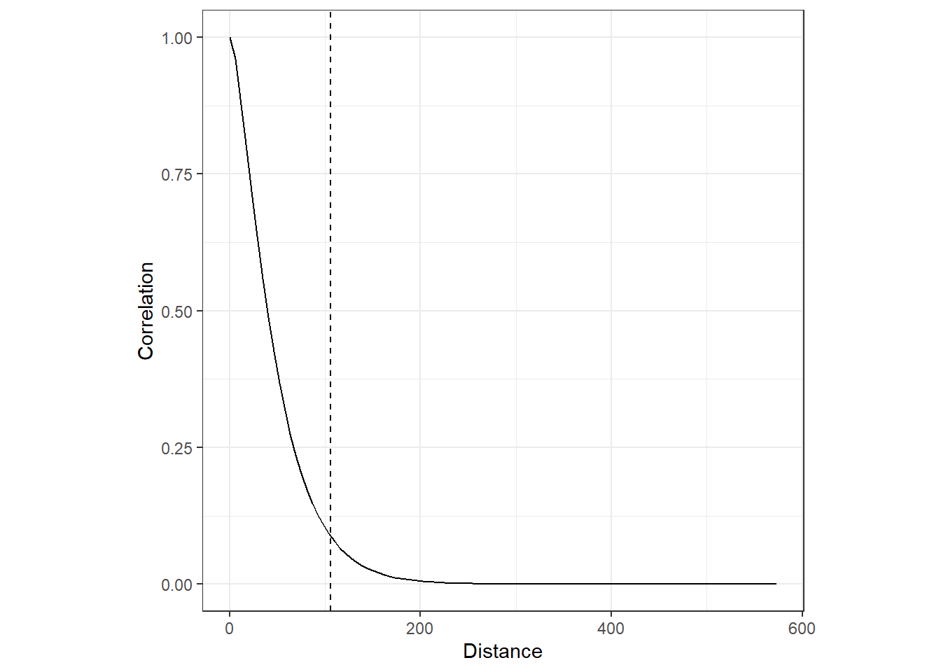

\(w_k\)の事後平均は以下のように求めることができる。

w.pm <- m12_2b$summary.random$w$mean

この\(w_k\)の事後平均をランダムガウス場に図示することができる。inla.mesh.projector関数はメッシュを用いて特定の範囲に格子を作成してくれる。通常はメッシュの最大最小の範囲に格子が作られる。

w.proj <- inla.mesh.projector(mesh12_5)

続いて、inla.mesh.projector関数で格子上にw.pmの事後平均を投影する。通常は、100×100の格子が用いられる。

w.pm100_100 <-inla.mesh.project(w.proj, w.pm)

最後に、格子状に\(w_k\)を図示する。

expand.grid(x = w.proj$x,
            y = w.proj$y) %>% 
  mutate(z = as.vector(w.pm100_100)) -> grid

ggplot(grid %>% drop_na(),
       aes(x = x, y = y))+
  geom_tile(aes(fill = z))+
  scale_fill_gradient2(high = muted("lightblue"), low = muted("pink"), mid = "white",
                       midpoint = -0.1)+
  geom_point(aes(x = Easting.km, y = Northing.km),
             data = iph,
             shape = 1)+
  stat_contour(aes(z = z, 
                   color = ..level..))+
  theme_bw()+
  theme(aspect.ratio = 1)+
  labs(x = "Easting(km)", y = "Northing(km)")+
  guides(color = "none")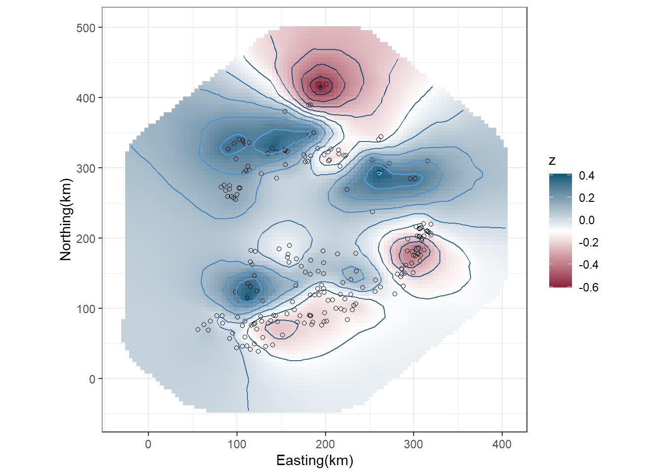

11.14 Model selection

WAICとDICを用いて、モデルに改善が見られなくなるまで1つずつ説明変数/交互作用項を除いていくという作業(step関数と同じ作業)を行っていく。まず、3次の交互作用項と2次の交互作用項を一つずつ除いたものを比較する。

## 3-way interractionなし  
f2c <- y ~ -1 + Intercept + Alt  + SDI + fFor + 
           Alt.SDI + Alt.fFor + SDI.fFor + f(w, model = spde)

Xc <- data.frame(Alt          = Xm[,2],
                SDI          = Xm[,3],
                fFor         = Xm[,4],
                Alt.SDI      = Xm[,5],
                Alt.fFor     = Xm[,6],
                SDI.fFor     = Xm[,7])

StackFitc <- inla.stack(
             tag = "Fit",
             data = list(y = iph$pH),  
               A = list(1, 1, A12_5),                  
               effects = list(   
                  Intercept = rep(1, N),
                  X = Xc,
                  w = w.index))

m12_2c <- inla(f2c,
               family = "gaussian",
               data = inla.stack.data(StackFitc),
               control.compute = list(dic = TRUE,
                                      waic = TRUE),
               control.predictor = list(A = inla.stack.A(StackFitc)))

## SDI.fForなし  
f2d <- y ~ -1 + Intercept + Alt  + SDI + fFor + 
           Alt.SDI + Alt.fFor + f(w, model = spde)

Xd <- data.frame(Alt          = Xm[,2],
                SDI          = Xm[,3],
                fFor         = Xm[,4],
                Alt.SDI      = Xm[,5],
                Alt.fFor     = Xm[,6])

StackFitd <- inla.stack(
             tag = "Fit",
             data = list(y = iph$pH),  
               A = list(1, 1, A12_5),                  
               effects = list(   
                  Intercept = rep(1, N),
                  X = Xd,
                  w = w.index))

m12_2d <- inla(f2d,
               family = "gaussian",
               data = inla.stack.data(StackFitd),
               control.compute = list(dic = TRUE,
                                      waic = TRUE),
               control.predictor = list(A = inla.stack.A(StackFitd)))

## Alt.fForなし
f2e <- y ~ -1 + Intercept + Alt  + SDI + fFor + 
           Alt.SDI +  SDI.fFor + f(w, model = spde)

Xe <- data.frame(Alt          = Xm[,2],
                SDI          = Xm[,3],
                fFor         = Xm[,4],
                Alt.SDI      = Xm[,5],
                SDI.fFor     = Xm[,7])

StackFite <- inla.stack(
             tag = "Fit",
             data = list(y = iph$pH),  
               A = list(1, 1, A12_5),                  
               effects = list(   
                  Intercept = rep(1, N),
                  X = Xe,
                  w = w.index))

m12_2e <- inla(f2e,
               family = "gaussian",
               data = inla.stack.data(StackFite),
               control.compute = list(dic = TRUE,
                                      waic = TRUE),
               control.predictor = list(A = inla.stack.A(StackFite)))

## Alt.SDIなし
f2f <- y ~ -1 + Intercept + Alt  + SDI + fFor + 
           Alt.fFor + SDI.fFor + f(w, model = spde)

Xf <- data.frame(Alt          = Xm[,2],
                SDI          = Xm[,3],
                fFor         = Xm[,4],
                Alt.fFor     = Xm[,6],
                SDI.fFor     = Xm[,7])

StackFitf <- inla.stack(
             tag = "Fit",
             data = list(y = iph$pH),  
               A = list(1, 1, A12_5),                  
               effects = list(   
                  Intercept = rep(1, N),
                  X = Xf,
                  w = w.index))

m12_2f <- inla(f2f,
               family = "gaussian",
               data = inla.stack.data(StackFitf),
               control.compute = list(dic = TRUE,
                                      waic = TRUE),
               control.predictor = list(A = inla.stack.A(StackFitf)))

その結果、3次の交互作用項と2次の交互作用項Alt.SDIを含まないモデルが最もWAICが低いことが分かった。一方で、DICは3次の交互作用のみを含まないモデルが最も低い。ここでは、m12_2fを採用することにする。

## モデル比較  
waic12_2 <- c(m12_2b$waic$waic, m12_2c$waic$waic, m12_2d$waic$waic, m12_2e$waic$waic, m12_2f$waic$waic)
dic12_2 <- c(m12_2b$dic$dic, m12_2c$dic$dic, m12_2d$dic$dic, m12_2e$dic$dic, m12_2f$dic$dic)
modelcomp12_2 <- cbind(waic12_2, dic12_2)
rownames(modelcomp12_2) <- c("Full","-Alt.SDI.fFor ", "-SDI.fFor", "-Alt.fFor","-Alt.SDI")

modelcomp12_2

##                waic12_2  dic12_2
## Full           127.7375 124.2912
## -Alt.SDI.fFor  126.5898 122.6982
## -SDI.fFor      127.6033 123.5803
## -Alt.fFor      133.1570 130.0797
## -Alt.SDI       126.5112 123.0979

続いて、残った2次の交互作用項を1つずつ除いたものと、交互作用項を含まないモデルとの比較を行う。

## Alt.fForなし
f2g <- y ~ -1 + Intercept + Alt  + SDI + fFor + 
            SDI.fFor + f(w, model = spde)

Xg <- data.frame(Alt          = Xm[,2],
                SDI          = Xm[,3],
                fFor         = Xm[,4],
                SDI.fFor     = Xm[,7])

StackFitg <- inla.stack(
             tag = "Fit",
             data = list(y = iph$pH),  
               A = list(1, 1, A12_5),                  
               effects = list(   
                  Intercept = rep(1, N),
                  X = Xg,
                  w = w.index))

m12_2g <- inla(f2g,
               family = "gaussian",
               data = inla.stack.data(StackFitg),
               control.compute = list(dic = TRUE,
                                      waic = TRUE),
               control.predictor = list(A = inla.stack.A(StackFitg)))

## SDI.fForなし
f2h <- y ~ -1 + Intercept + Alt  + SDI + fFor + 
           Alt.fFor  + f(w, model = spde)

Xh <- data.frame(Alt          = Xm[,2],
                SDI          = Xm[,3],
                fFor         = Xm[,4],
                Alt.fFor     = Xm[,6])

StackFith <- inla.stack(
             tag = "Fit",
             data = list(y = iph$pH),  
               A = list(1, 1, A12_5),                  
               effects = list(   
                  Intercept = rep(1, N),
                  X = Xh,
                  w = w.index))

m12_2h <- inla(f2h,
               family = "gaussian",
               data = inla.stack.data(StackFith),
               control.compute = list(dic = TRUE,
                                      waic = TRUE),
               control.predictor = list(A = inla.stack.A(StackFith)))

## 交互作用なし
f2i <- y ~ -1 + Intercept + Alt  + SDI + fFor + f(w, model = spde)

Xi <- data.frame(Alt          = Xm[,2],
                SDI          = Xm[,3],
                fFor         = Xm[,4])

StackFiti <- inla.stack(
             tag = "Fit",
             data = list(y = iph$pH),  
               A = list(1, 1, A12_5),                  
               effects = list(   
                  Intercept = rep(1, N),
                  X = Xi,
                  w = w.index))


m12_2i <- inla(f2i,
               family = "gaussian",
               data = inla.stack.data(StackFiti),
               control.compute = list(dic = TRUE,
                                      waic = TRUE),
               control.predictor = list(A = inla.stack.A(StackFiti)))

その結果、わずかながら2次の交互作用項を2つ含むモデル(m12_2f)が最もWAICとDICが低いことが分かった。

## モデル比較  
waic12_2 <- c(m12_2f$waic$waic, m12_2g$waic$waic, m12_2h$waic$waic, m12_2i$waic$waic)
dic12_2 <- c(m12_2f$dic$dic, m12_2g$dic$dic, m12_2h$dic$dic, m12_2i$dic$dic)
modelcomp12_2 <- cbind(waic12_2, dic12_2)
rownames(modelcomp12_2) <- c("Full","-Alt.fFor ", "-SDI.fFor", "no interaction")

modelcomp12_2

##                waic12_2  dic12_2
## Full           126.5112 123.0979
## -Alt.fFor      130.7929 128.1620
## -SDI.fFor      126.8899 123.4883
## no interaction 133.8153 131.2625

11.15 Model validation

続いて、モデル診断を行う。

まず、残差と予測値を計算する。m12_2f$summary.fitted.valuesはデータ数210ではなく合計632行のデータを返すが、最初の210個が予測値である。残りの432個が何を示しているのかは後ほど触れる。

fitted <- m12_2f$summary.fitted.values$mean[1:210]
resid <- iph$pH - fitted

残差と予測値、残差と共変量の関係を見ると、1つだけ外れ値があるものの、全体的なパターンはないように見える。

data.frame(fitted = fitted,
           resid = resid) %>% 
  ggplot(aes(x= fitted, y = resid))+
  geom_point(shape = 1)+
  geom_hline(yintercept = 0, linetype = "dashed")+
  theme_bw()+
  theme(aspect.ratio = 1)+
  labs(x= "Fitted values", y = "Residuals") -> p1

data.frame(SDI = iph$SDI,
           resid = resid) %>% 
  ggplot(aes(x= SDI, y = resid))+
  geom_point(shape = 1)+
  geom_hline(yintercept = 0, linetype = "dashed")+
  theme_bw()+
  theme(aspect.ratio = 1)+
  labs(x= "SDI", y = "Residuals") -> p2

data.frame(SDI = iph$logAlt,
           resid = resid) %>% 
  ggplot(aes(x= SDI, y = resid))+
  geom_point(shape = 1)+
  geom_hline(yintercept = 0, linetype = "dashed")+
  theme_bw()+
  theme(aspect.ratio = 1)+
  labs(x= "Log(Altitude)", y = "Residuals") -> p3

data.frame(forested = iph$fForested,
           resid = resid) %>% 
  ggplot(aes(x= forested, y = resid))+
  geom_boxplot()+
  theme_bw()+
  theme(aspect.ratio = 1)+
  labs(x= "Forested", y = "Residuals") -> p4

(p1 + p2)/(p3+p4)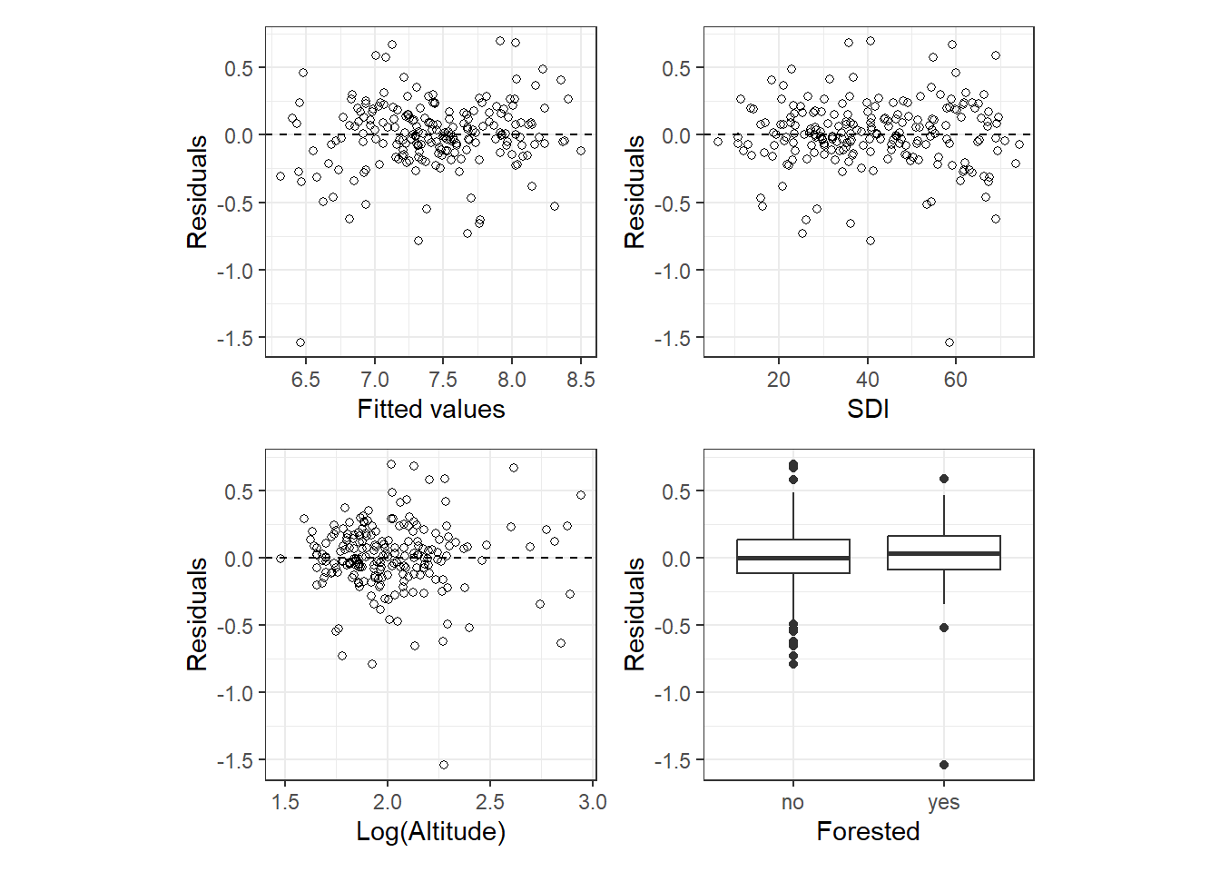

続いて、バリオグラムを確認する。空間的相関を考慮しなかった場合に比べると水平に近づいており、改善しているように見える。

vario_12_2f <- data.frame(resid = resid,
                          Easting.km = iph$Easting/1000,
                          Northing.km = iph$Northing/1000)

sp::coordinates(vario_12_2f) <- c("Easting.km", "Northing.km")

vario_12_2f %>% 
  variogram(resid ~ Easting.km + Northing.km, data = .,
            ## 0が南北方向、90が東西方向
            alpha = c(0, 90),
            cressie = TRUE,
            cutoff = 150,
            width = 10) %>% 
  ggplot(aes(x = dist, y = gamma))+
  geom_point(aes(size = np))+
  theme_bw()+
  theme(aspect.ratio = 1)+
  facet_rep_wrap(~ dir.hor,
                 labeller = as_labeller(c("0" = "North-South",
                                          "90" = "East-West")),
                 repeat.tick.labels = TRUE)+
  labs(y = "semivariogram")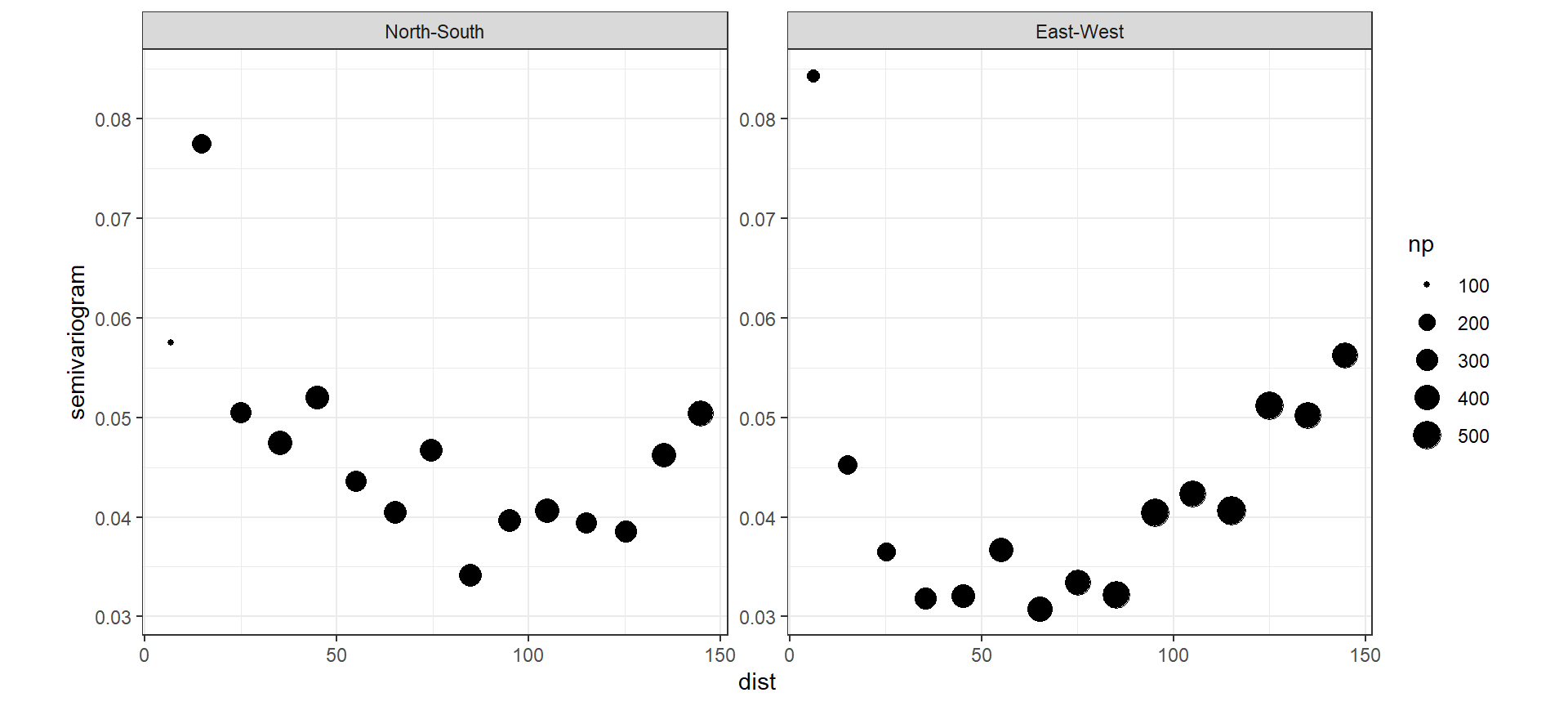

11.16 Model interpretation

選ばれたモデルの結果は以下のとおりである。

m12_2f$summary.fixed %>% 
  print(digits = 2)

##             mean     sd 0.025quant 0.5quant 0.975quant   mode     kld
## Intercept  8.114 0.2996      7.522    8.115      8.700  8.117 5.6e-09
## Alt        0.162 0.1432     -0.119    0.163      0.443  0.163 6.5e-10
## SDI       -0.023 0.0022     -0.028   -0.023     -0.019 -0.023 2.5e-09
## fFor       1.117 0.3971      0.336    1.117      1.895  1.118 6.2e-10
## Alt.fFor  -0.484 0.1912     -0.859   -0.484     -0.109 -0.484 6.7e-10
## SDI.fFor  -0.004 0.0041     -0.012   -0.004      0.004 -0.004 5.4e-10

inla.emarginal(function(x) 1/sqrt(x), m12_2f$marginals.hyperpar$`Precision for the Gaussian observations`)

## [1] 0.2900052

モデル式に当てはめると以下のようになる。
\[ \begin{aligned} &pH_i \sim N(\mu_i, 0.29^2)\\ &E(pH_i) = \mu_i \; and \; var(pH_i) = 0.29^2\\ &\mu_i = \begin{cases} 9.23 -0.027 \times SDI_i + -0.321 \times logAltitude_i + u_i & \rm{if \; not \; forested} \\ 8.12 -0.023 \times SDI_i + 0.162 \times logAltitude_i + u_i & \rm{if \; forested}\\ \end{cases} \end{aligned} \]

INLAで時空間モデルの予測値とその95%確信区間を得るには、前章までとは少し違う工夫が必要がある。予測値が欲しい範囲の変数と応答変数がNAであるデータフレームを作るのは同様だが、それを”stack”オブジェクトにする必要がある。

newdata <- crossing(logAlt = seq(min(iph$logAlt), max(iph$logAlt), length = 100),
                    SDI = seq(min(iph$SDI), max(iph$SDI), length = 100),
                    fForested = iph$fForested)

Xmm <- model.matrix(~ logAlt*fForested + SDI * fForested, 
                   data = newdata)

Xp <- data.frame(Alt = Xmm[,2],
                 SDI = Xmm[,4],
                 fFor = Xmm[,3],
                 Alt.fFor = Xmm[,5],
                 SDI.fFor = Xmm[,6])

StackCov <- inla.stack(
  tag = "Covariates",
  data = list(y = NA),
  A = list(1,1),
  effects = list(
    Intercept = rep(1, nrow(newdata)),
    Xp = Xp))

作成した”stack”オブジェクトはもともとのオブジェクトに結合する。

All.stack <- inla.stack(StackFitf, StackCov)

その後、結合したものでモデルを実行する。その後は基本的に空間的相関を考慮しない場合と同じである。結果を図示したのが以下の図である。

f2fit <- y ~ -1 + Intercept + Alt  + SDI + fFor + 
           Alt.fFor + SDI.fFor + f(w, model = spde)

m12_2fit <- inla(f2fit,
                 family = "gaussian",
                 data = inla.stack.data(All.stack),
                 control.compute = list(dic = TRUE,
                                      waic = TRUE),
                 control.predictor = list(A = inla.stack.A(All.stack)))

## 何番目から何番目の値がnewdataの予測値か
index.cov <- inla.stack.index(All.stack,
                              tag = "Covariates")$data


## 予測値と95%確信区間  
fit12_2 <- bind_cols(newdata,
                     m12_2fit$summary.fitted.values[index.cov, c(1,3,5)])

## 図示  
plot_ly(fit12_2 %>% group_by(fForested),
        x = ~logAlt,
        y = ~SDI,
        z = ~mean,
        size = 2,
        type = "surface",
        colors = c("black","grey"),
        alpha = 0.2) %>% 
  add_markers(color = ~fForested)

続いて、地図上にランダム切片\(u_i\)を図示する。まずは、\(u_i\)を算出する。これは、式(11.2)より\(\bf{u} = \bf{A} \times \bf{w}\)であることを利用して簡単に求められる。

## uの算出
w.pm <- m12_2f$summary.random$w$mean
u <- as.matrix(A12_5) %*% w.pm

## 格子上にwkの値を投影  
w.proj <- inla.mesh.projector(mesh12_5)
w.pm100_100 <-inla.mesh.project(w.proj, w.pm)

続いて、求めた値を地図上に図示したものが図11.3である。

## EastingとNorthingを緯度と経度に変換
sp_u <- SpatialPointsDataFrame(coords = cbind(iph$Easting, iph$Northing),
                               data = data.frame(u = u,
                                                 ID = iph$ID,
                                                 pH = iph$pH),
                                proj4string = CRS("+init=epsg:29902"))

sp_u_data <- spTransform(sp_u, CRS("+init=epsg:4322"))

## アイルランドの地図をダウンロード
Ireland <- st_read("shpfile/IRL_adm0.shp")

## Reading layer `IRL_adm0' from data source 
##   `C:\Users\Tsubasa Yamaguchi\Desktop\R_studies\practice\Spatial-temporal_analysis\shpfile\IRL_adm0.shp' 
##   using driver `ESRI Shapefile'
## Simple feature collection with 1 feature and 70 fields
## Geometry type: MULTIPOLYGON
## Dimension:     XY
## Bounding box:  xmin: -10.66305 ymin: 51.41958 xmax: -5.993611 ymax: 55.45042
## Geodetic CRS:  WGS 84

Ireland.sf <- st_transform(Ireland, crs = 4322)


## 図示
st_as_sf(sp_u_data) %>% 
  ggplot()+
  geom_sf(data = Ireland.sf,
          fill = "darkgreen")+
  geom_sf(aes(size = abs(u),
              color = u <= 0,
              shape = u <= 0),
          alpha = 0.7)+
  scale_size(range = c(0.01,4))+
  scale_shape_manual(values = c(17,16))+
  scale_color_manual(values = c("yellow1","red3"))+
  theme_bw()+
  labs(color = "u > 0",
       shape = "u > 0",
       size = "abs(u)")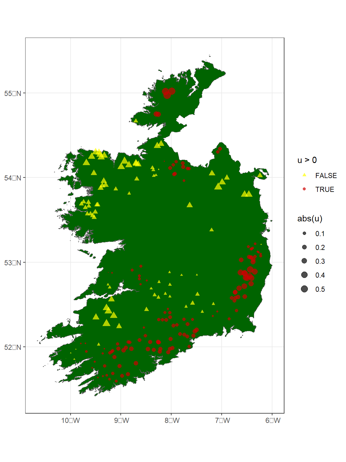

図11.3: Map of Ireland with estimated us.

ランダムガウス場上に推定された\(u_i\)をプロットすると以下のようになる。

grid_w <- expand.grid(x = w.proj$x,
                      y = w.proj$y) %>% 
  mutate(w = as.vector(w.pm100_100))

df_u <- data.frame(x = iph$Easting.km,
                   y = iph$Northing.km,
                   u = u)

ggplot(grid_w %>% drop_na(),
        aes(x = x, y = y))+
  stat_contour(aes(z = w, 
                   color = ..level..),
               linewidth = 1)+
  scale_color_gradient2(high = muted("green2"), low = muted("red"), mid = "yellow",
                        midpoint = 0)+
  geom_point(data = df_u,
             aes(size = abs(u),
                 shape = u > 0),
             alpha = 0.7)+
  scale_size(range = c(0.01,4))+
  scale_shape_manual(values = c(17,16))+
  theme_bw()+
  theme(aspect.ratio = 1)+
  labs(x = "Easting(km)", y = "Northing(km)")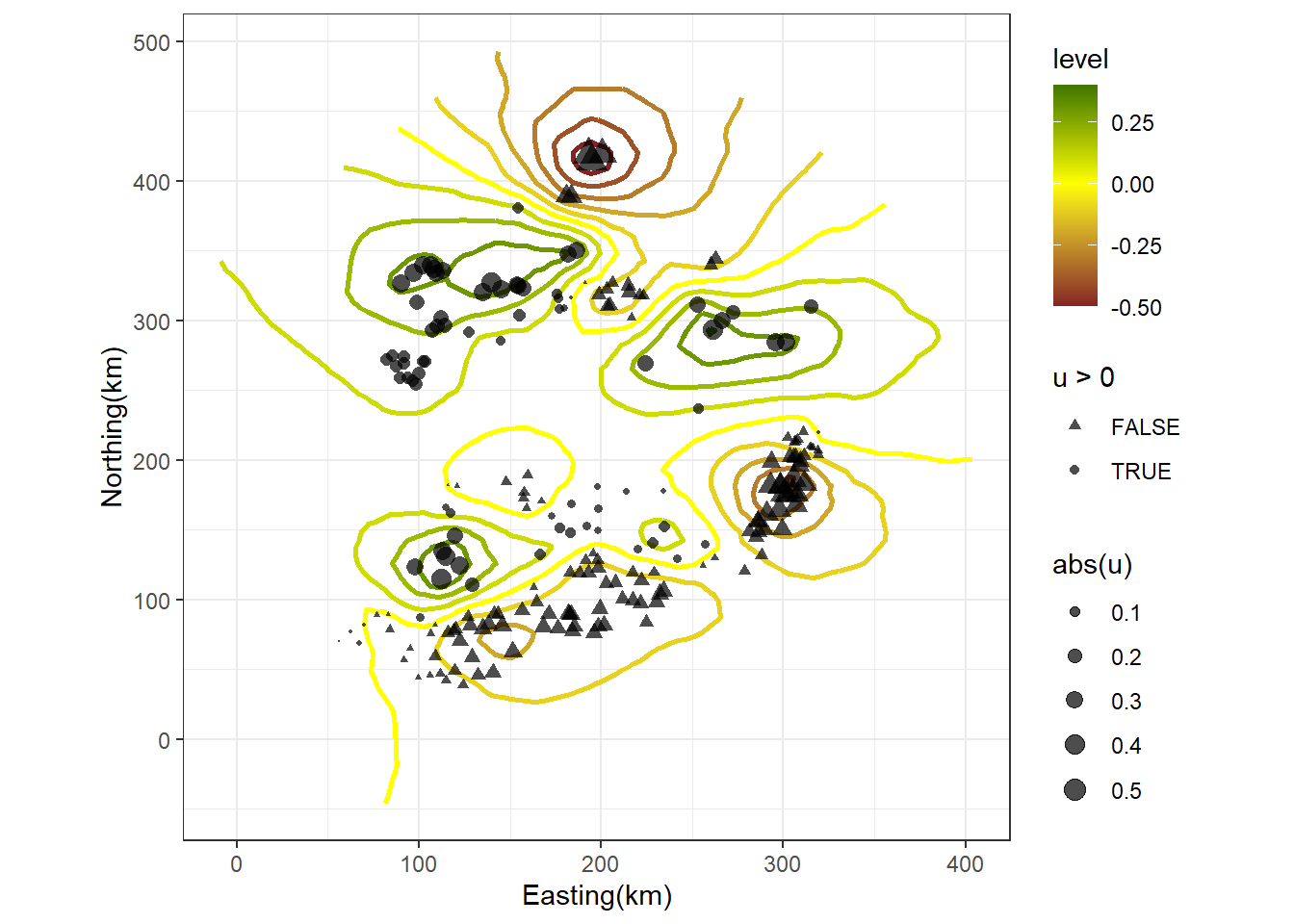

11.17 Detailed information about the stack

以下では、どのように予測値を得ていたのかを解説する。

11.17.1 Stack for the fitted model again

メッシュ(mesh12_5)は737個の頂点を持つので、A12_5は、\(a_{ik}\)を含む行列\(\bf{A}\)である(式(11.2)参照)。

dim(A12_5)

## [1] 210 737

各行は各データに対応する。すなわち、A12_5[1,]は\(a_{1k}\)に対応する。前章(10)で見たように、もしデータのサンプリングポイント\(i\)(\(s_i\))が頂点\(k\)上にあれば\(a_{ik} = 1\)、なければ\(a_{ik} = 0\)である。また、もし\(s_i\)が三角形内にある場合はその三角形の頂点の\(a_{ik}\)には0から1の間の小数値が合計1になるように割り振られる。よって、\(\bf{A}\)(A12_5)の各行の合計は1になる。

空間的相関を考慮したモデルの式は以下のように書ける。
\[ \begin{aligned} \bf{\mu} &= \rm{Intercept} + \rm{Covariates} + \rm{Spatial \;random \;effects}\\ &= \bf{A_1} \times \rm{Intercept} + \bf{A_2} \times \rm{Covariates} + \bf{A_3} \times \rm{Spatial \;field} (\bf{w})\\ &= \begin{pmatrix} \bf{A_1} & \bf{A_2} & \bf{A_3} \end{pmatrix} \times \begin{pmatrix} \rm{Intercept}\\ \rm{Covariates}\\ \rm{Spatial field} (\bf{w}) \end{pmatrix} \\ &= \bf{A} \times \bf{Z} \end{aligned} \]

ここで、\(\bf{A_1,A_2,A_3}\)はそれぞれモデルを回すときにinla.stack関数のA =で指定したものである(今回はそれぞれ1, 1, A12_5)。\(\bf{A_1}\)は全てが1の210行×1列の行列、\(\bf{A_2}\)は210行×210列の単位行列である。行列\[\bf{A} = \begin{pmatrix} \bf{A_1} & \bf{A_2} & \bf{A_3} \end{pmatrix}\]は、以下のように求められる。

A <- inla.stack.A(StackFitf)

dim(A)

## [1] 210 422

ここには列数が\(1 + 210 + 737 = 948\)ではなく422列しかない。これは、INLAが\(\bf{A_3}\)のうち合計が0である列を計算しないからである。以下で計算しているように列の合計が0より大きいものは211列なので、\(1 + 210 + 211 = 422\)列になるのである。

table(colSums(A12_5) > 0)

## 
## FALSE  TRUE 
##   526   211

11.17.2 Stack for the new covariate values

新しい共変量の値に対してモデルの予測値を得る場合には、前節(11.16)でやったように予測をしたい範囲の共変量を含むデータフレームを作成し、“stack”オブジェクトを作成する必要がある。このとき、応答変数はNAにする。ここで、A = list(1,1)とするのはモデルの予測には空間的相関を考慮する項\(u_i\)を含まないため、\(\bf{A_3}\)が必要ないからである。

Xmm <- model.matrix(~ logAlt*fForested + SDI * fForested, 
                   data = newdata)

Xp <- data.frame(Alt = Xmm[,2],
                 SDI = Xmm[,4],
                 fFor = Xmm[,3],
                 Alt.fFor = Xmm[,5],
                 SDI.fFor = Xmm[,6])

StackPred <- inla.stack(
    tag = "Predict",
    data = list(y = NA),
    A = list(1,1),
    effects = list(
    Intercept = rep(1, nrow(newdata)),
    Xp = Xp))

ここで、もともとモデルを実行するときに用いていた\(\bf{A}\)を\[\bf{A^1} = \begin{pmatrix} \bf{A^1_1} & \bf{A^1_2} & \bf{A^1_3} \end{pmatrix}\]、予測に用いる\(\bf{A}\)を\[\bf{A^2} = \begin{pmatrix} \bf{A^2_1} & \bf{A^2_2} \end{pmatrix}\]とする。このとき、モデルフィットのためのモデル式は以下のように書ける。

\[ \begin{aligned} \bf{\mu^1} &= \begin{pmatrix} \bf{A^1_1} & \bf{A^1_2} & \bf{A^1_3} \end{pmatrix} \times \begin{pmatrix} \rm{Intercept}\\ \rm{Covariates}\\ \rm{Spatial field} (\bf{w}) \end{pmatrix} \\ &= \bf{A^1} \times \bf{Z^1} \end{aligned} \tag{11.4} \]

一方、予測値を得るためのモデル式は以下のように書ける。
\[ \begin{aligned} \bf{\mu^2} &= \begin{pmatrix} \bf{A^2_1} & \bf{A^2_2} \end{pmatrix} \times \begin{pmatrix} \rm{Intercept}\\ \rm{Covariates}\\ \end{pmatrix} \\ &= \bf{A^2} \times \bf{Z^2} \end{aligned} \tag{11.5} \]

newdataは20000行なので、\(\bf{A^2_1}\)は20000行×1列、\(\bf{A^2_2}\)は20000行×20000列である。よって、\(\bf{A^2}\)は20000行×20001列になる。

dim(inla.stack.A(StackPred))

## [1] 20000 20001

11.17.3 Combine the two stacks

続いて、モデルフィットのための”stack”(StackFitf)と予測のための”stack”(StackPred)を結合する。

All.stack <- inla.stack(StackFitf, StackPred)

このとき、式(11.4)と式(11.5)が結合され以下のように書ける。
\[ \begin{aligned} \begin{pmatrix} \mu^1 \\ \mu^2 \end{pmatrix} &= \begin{pmatrix} \bf{A^1} & 0 \\ 0 & \bf{A^2} \end{pmatrix} \times \begin{pmatrix} \bf{Z^1} \\ \bf{Z^2} \end{pmatrix} \\ &= \bf{A} \times \bf{Z} \end{aligned} \]

よって、All.stackの行数はStackFitfとStackPredの行数を足し合わせたものになる。列数については、列数の合計から1を引いた値になっている(重複しているInterceptを除いている)。

dim(inla.stack.A(All.stack))

## [1] 20210 20422

11.17.4 Run the model

最後に、結合した”stack”を用いてモデルを実行する。

f2fit <- y ~ -1 + Intercept + Alt  + SDI + fFor + 
           Alt.fFor + SDI.fFor + f(w, model = spde)

m12_2fit <- inla(f2fit,
                 family = "gaussian",
                 data = inla.stack.data(All.stack),
                 control.compute = list(dic = TRUE,
                                      waic = TRUE),
                 control.predictor = list(A = inla.stack.A(All.stack)))

モデルの予測値は40632行ある。これは、summary.fitted.valuesが”stack”オブジェクト(All.stack)の全ての要素について予測値を算出するからである。40632はAll.stackの行数と列数を足したものである。

dim(m12_2fit$summary.fitted.values)

## [1] 40632     6

inla.stack.index関数を用いれば、何行目に目当ての予測値があるかを容易に知ることができる。実データについての予測値は以下のように抽出できる。

index.fit <- inla.stack.index(All.stack,
                              tag = "Fit")$data

fit12_2_raw <- m12_2fit$summary.fitted.values[index.fit, c(1,3,5)]

新しい共変量の値に対してモデルの予測値を得る場合は以下のように抽出できる。

index.predict <- inla.stack.index(All.stack,
                                  tag = "Predict")$data

fit12_2_predict <- m12_2fit$summary.fitted.values[index.predict, c(1,3,5)]

References

Cruikshanks R, Lauridsen R, Harrison A, et al (2006) Evaluation of the use of the sodium dominance index as a potential measure of acid sensitivity