6 Generalized Additive Models applied on northern gannets
6.1 Northern Gannet in the north sea
Camphuysen and Powell は北海のキタカツオドリ(Morus bassanus)を対象に探索採食戦術の研究を行った。研究では300m幅のトランゼクトで確認された個体数が記録されている。リサーチクエスチョンは、カツオドリはいつコロニーの近くで採食をするのかである。
6.2 The variables
データは以下の通り。各行のデータが各トランゼクトのデータを表している。目的変数はトランゼクト内のカツオドリの数である。
Day: 観察した日
Month: 観察した月
Year: 観察した年
Hours: 観察時の時間
Minutes: 観察時の分
Latitude、Y: 緯度
Longtitude、X: 経度
Area_surveyedkm2: 探索エリアの面積
Seastate: 海の状態
Gannets_in_transect: トランゼクト内のカツオドリの数
6.3 Brainstorming
まず、データを収集したトランゼクトの場所が年ごとに違っていないかを確かめる。図6.1を見る限りは概ね同じエリアでデータが採集されていたことが分かる。
Gannets %>%
  ggplot(aes(x = Longitude, y = Latitude))+
  geom_count(alpha = 0.5)+
  theme_bw()+
  theme(aspect.ratio = 1.5)+
  facet_rep_wrap(~Year, repeat.tick.labels = TRUE,
                 ncol = 5)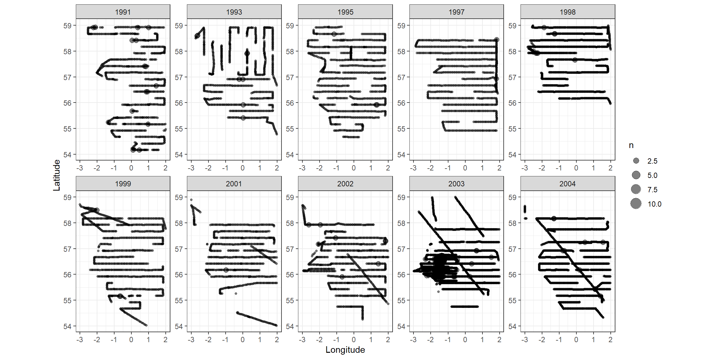
図6.1: Spatial position of each transect per year.
最初に考えなければならないのは、トランゼクトごとに探索努力が異なるということである。探索努力はトランゼクトのサイズとして定量化されている。図6.2を見るとトランゼクトのサイズは大きくばらついているので、これを考慮する必要がある。
Gannets %>%
  mutate(no_samples = 1:n()) %>%
  ggplot(aes(x = Area_surveyedkm2, y = no_samples))+
  geom_point(alpha = 0.5)+
  theme_bw()+
  theme(aspect.ratio = 1)+
  labs(x = "Area", y = "Order of the data")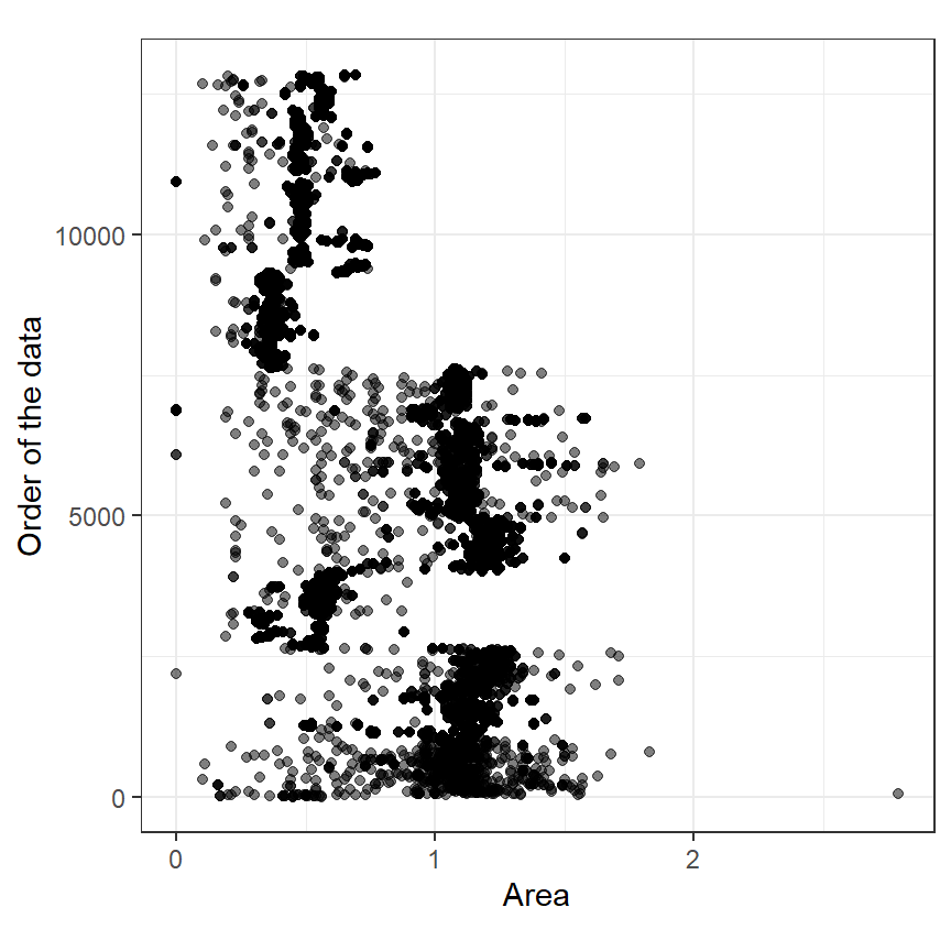
図6.2: Clevela nd dotplot illustrating the sizes of the transects.
第4章で見たように、もしトランゼクトサイズが10倍になったら確認できる鳥の数も10倍になると考えられるなら、トランゼクトサイズの対数をオフセット項として含めることができる。一方で、もしそうでないならばトランゼクトサイズは共変量として説明変数に含める必要がある。今回はオフセット項で用いるが、サイズが0のもの(定点観測を行ったデータ)も存在するので、それは除外する。また、時刻を表す列も作成する。また、1年の中でのユリウス通日(1月1日からの経過日数)と1991年1月1日からの経過日数も算出する。
Gannets %>%
  filter(Area_surveyedkm2 > 0) %>%
  mutate(LArea = log(Area_surveyedkm2)) %>%
  mutate(Time = Hours + Minutes/60) %>%
  mutate(Xkm = X/1000, Ykm = Y/1000) %>%
  mutate(Date = as.POSIXct(str_c(Year,"-",Month,"-",Day))) %>%
  ## 年内のユリウス通日
  mutate(DayInYear = strptime(Date, "%Y-%m-%d")$yday + 1) %>%
  ## 1991年1月1日からの経過日数
  mutate(DaySince0 = ceiling(julian(strptime(Date, format = "%Y-%m-%d"), orogin = as.Date("1991-01-01")))) %>%
  rename(G = Gannets_in_transect) -> Gannets2
データは1991年から2004年の6から7月、4時から20時間に収集されている。カツオドリの数は年と日付、時間、トランゼクトの位置によって異なる。そこで、以下のモデル式を考える。このモデルは日付の効果は年に依らず同じで、時間の効果は年や月に依らずに同じで、トランゼクトの位置の効果は時間によって変化しないことを仮定している(= 交互作用を入れていない)。調査は6月と7月にしか行われていないので、日付の効果が時間によって変わらないという仮定は妥当だろう。これは、\(f(Day_i, Hour_i)\)を含めないということを意味する。
\[ \begin{aligned} G_i &\sim Poisson(\mu_i)\\ log(\mu_i) &= \alpha + f_1(Year) + f_2(Day_i) + f_3(Hours_i) + f_4(X_i,Y_i) + \beta \times SeaState_i + log(Area_i) \end{aligned} \]
もしトランゼクトの場所の効果が年によって異なると仮定するなら、以下のようなモデルになる。
\[
\begin{aligned}
G_i &\sim Poisson(\mu_i)\\
log(\mu_i) &= \alpha + f_1(Year, X_i, Y_i) + f_2(Day_i) + f_3(Hours_i) + \beta \times SeaState_i + log(Area_i)
\end{aligned}
\]
ひとまず、以下ではデータ探索を行ったうえで、最も適切だと思えるモデルを考えていく。
6.4 Data exploration
図6.3は、地点ごとのカツオドリの密度を点の大きさで表したものである。年によって密度が高い場所は異なっているように見える。これは、\(f(Priod_1, X_i, Y_i)\)という3次元smootherが必要であることを示唆している。
Gannets2 %>%
  mutate(Density = G/Area_surveyedkm2) %>%
  ggplot(aes(x = Xkm, y = Ykm))+
  geom_point(aes(size = Density),
             alpha = 0.7)+
  scale_size(range = c(0,12))+
  theme_bw()+
  theme(aspect.ratio = 1.5)+
  facet_rep_wrap(~Year, repeat.tick.labels = TRUE,
                 ncol = 4)+
  labs(x = "Xkm", y = "Ykm")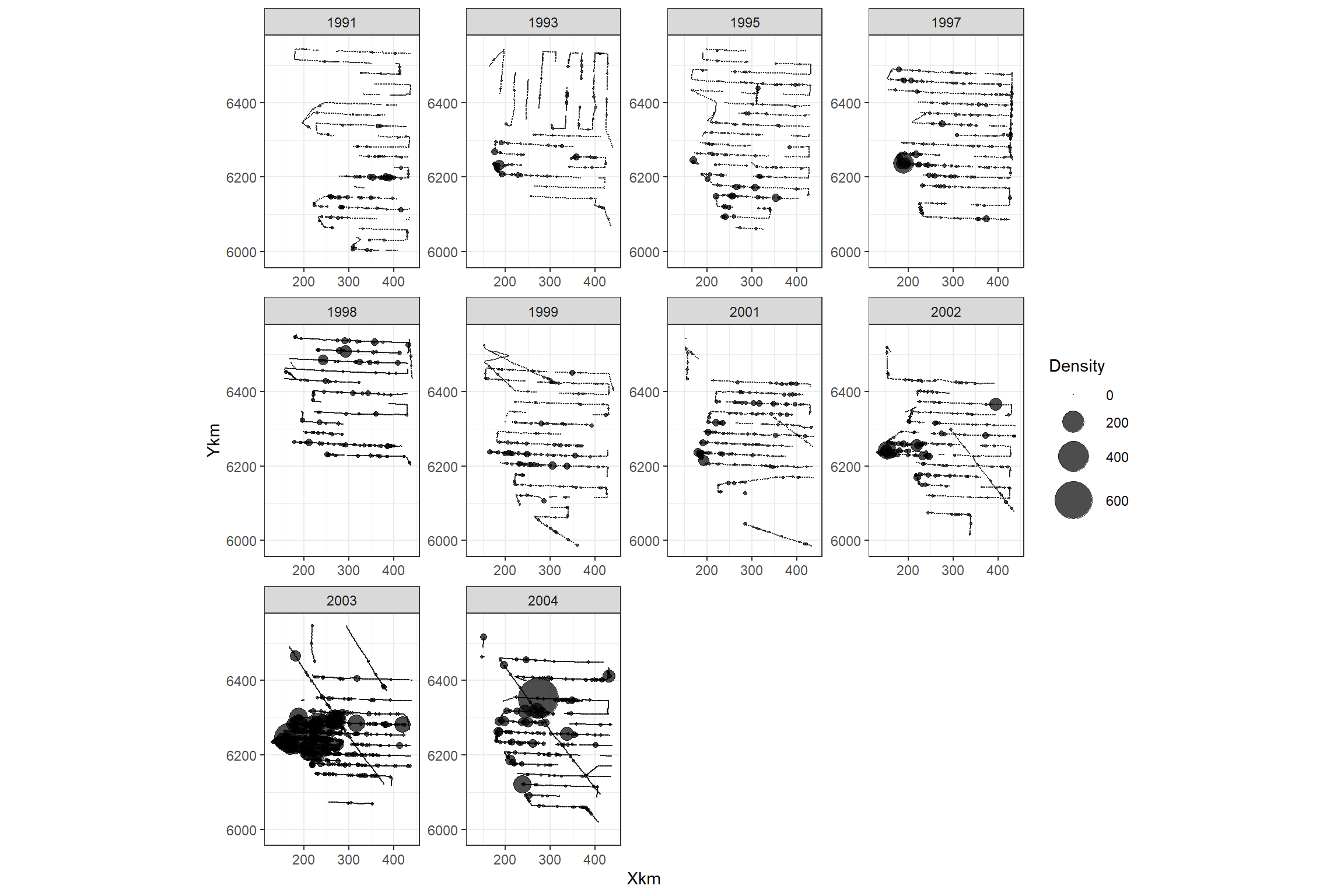
図6.3: Gannet density plotted versus spatial coordinates and year. The size of a dot is proportional to the gannet density.
図6.4は、時間とその年の1月1日からの経過日数によって密度がどのように異なるかを年ごとに可視化したものである。年によって密度が高い日や時間帯が異なっていることが分かる。
Gannets2 %>%
  mutate(Density = G/Area_surveyedkm2) %>%
  ggplot(aes(x = Hours, y = DayInYear))+
  geom_point(aes(size = Density),
             alpha = 0.7)+
  scale_size(range = c(0,12))+
  theme_bw()+
  theme(aspect.ratio = 1.5)+
  facet_rep_wrap(~Year, repeat.tick.labels = TRUE,
                 ncol = 4)+
  labs(x = "Hour", y = "Day")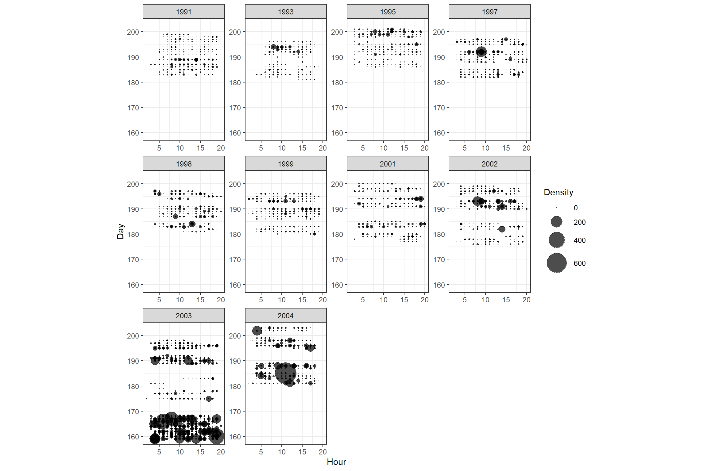
図6.4: Gannet density plotted versus hour, day, and year. The size of a dot is proportional to the gannet density.
また、データにゼロ過剰がないかも確認する必要がある。カツオドリの数が0のデータは全体の0.81に及ぶ。もしモデルが仮定するよりも過剰にゼロがあると過分散の問題を引き起こすので、ゼロ過剰モデルを適用する必要がある。まずは普通のポワソン分布を適用し、ゼロ過剰でないかを確認する。
多重共線性の問題も考える必要がある。例えば、時刻や日付が海の状態と関連している可能性はあるが、図6.5を見る限りは問題なさそう。
Gannets2 %>%
  dplyr::select(Time, DayInYear, Seastate) %>%
  pivot_longer(1:2) %>%
  mutate(Seastate = as.factor(Seastate)) %>%
  ggplot(aes(x = Seastate, y = value))+
  geom_boxplot()+
  facet_rep_wrap(~name, repeat.tick.labels = TRUE, scales = "free_y")+
  theme_bw()+
  theme(aspect.ratio = 1.2)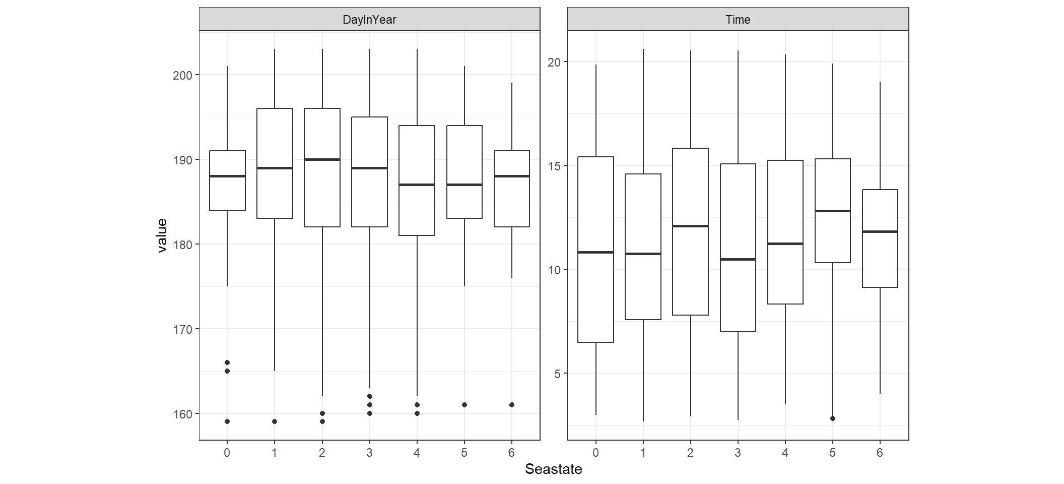
図6.5: Boxplot of Time conditional on Seastate and DayInYear conditional on Seastate.
確認されたカツオドリの数を見てみると、いくつかかなり大きいものがあることが分かる。また、前述したように0が多い。次節ではまずポワソン分布のGAMから入るが、おそらくゼロ過剰負の二項分布のGAMを適用する必要があると思われる。
Gannets2 %>%
  mutate(no_samples = 1:n()) %>%
  ggplot(aes(x = G, y = no_samples))+
  geom_point(alpha = 0.5)+
  theme_bw()+
  theme(aspect.ratio = 1)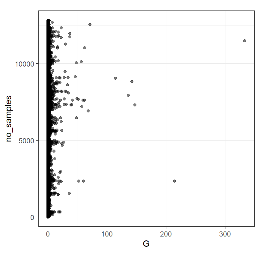
図6.6: Cleveland dotplot of gannet abundance.
6.5 Building up the complexity of the GAMs
まずはポワソン分布のGAMを適用する。GLMではなくGAMを適用するのは、日付や月、年による変化は明確に非線形だからである。まずは年のsmootherだけを含む以下のモデルを考える。\(G_i\)は確認されたカツオドリの数、\(LSA_i\)はトランゼクトのサイズの対数である。
\[ \begin{aligned} G_i &\sim Poisson(\mu_i)\\ log(\mu_i) &= \alpha + f_1(Year_i) + LSA_i \\ \end{aligned} \]
Rでは以下のように実行する。
まずは過分散を確認する。分散パラメータ\(\phi\)を算出すると(第4.4節参照)、高い数値をとっており、過分散が生じていることが分かる。
## [1] 36.92865ゼロ過剰モデルや負の二項分布モデルを考える前に、他の共変量を加えることで過分散が解決するかを確認する。次は海の状態を加えた以下のモデルを考える。
\[ \begin{aligned} G_i &\sim Poisson(\mu_i)\\ log(\mu_i) &= \alpha + f_1(Year_i) + \beta \times Seastate_i + LSA_i \\ \end{aligned} \]
Rでは以下のように実行する。
分散パラメータ\(\phi\)を計算すると、まだ過分散は解決されていない。
## [1] 29.7664続いて、時刻のsmootherも追加したモデルを考える。
\[
\begin{aligned}
G_i &\sim Poisson(\mu_i)\\
log(\mu_i) &= \alpha + f_1(Year_i) + f_2(Times_i) + \beta \times Seastate_i + LSA_i \\
\end{aligned}
\]
Rでは以下のように実行する。
M6_3 <- gam(G ~ s(Year) + s(Time) + offset(LArea) + factor(Seastate),
family = poisson, data = Gannets2)分散パラメータ\(\phi\)を計算すると、まだ過分散は解決されていない。
## [1] 26.70897続いて、1年の中での経過年数のsmootherもモデルに加える。
\[
\begin{aligned}
G_i &\sim Poisson(\mu_i)\\
log(\mu_i) &= \alpha + f_1(Year_i) + f_2(Times_i) + f_3(DayInYear_i) + \beta \times Seastate_i + LSA_i \\
\end{aligned}
\]
Rでは以下のように実行する。
M6_4 <- gam(G ~ s(Year) + s(Time) + s(DayInYear) + offset(LArea) + factor(Seastate),
family = poisson, data = Gannets2)分散パラメータ\(\phi\)を計算すると、まだ過分散は解決されていない。
## [1] 23.05207次に、緯度と経度の2次元smootherも追加する。
\[
\begin{aligned}
G_i &\sim Poisson(\mu_i)\\
log(\mu_i) &= \alpha + f_1(Year_i) + f_2(Times_i) + f_3(DayInYear_i) + f_4(X_i,Y_i) + \beta \times Seastate_i + LSA_i \\
\end{aligned} \tag{6.1}
\]
Rでは以下のように実行する。GAMではそれぞれのsmootherに罰則が与えられているが、2次元smootherの2つの共変量はそれぞれ同様に罰則を与えられるべきである。特に、二つの共変量が異なるスケールを持つときにはこれに気を付ける必要がある。このようなときは、いわゆる非等方性スムーザー(non-isotopic smoother)を用いるべきである。ここでは、テンソル積smoother(te())を用いる。これについては、こちらが詳しい。テンソル積smootherは、異なるスケールを持つ共変量の2次元smootherを用いる場合に有用である。ただし、2つの共変量が同じスケールを持つ場合にはs()を用いる方がよいようである。今回はXkmとYkmが異なるスケールを持つため、テンソル積smootherを用いる。
Rでは以下のように実行する。
M6_5 <- gam(G ~ s(Year) + s(Time) + s(DayInYear) + te(Xkm, Ykm) + offset(LArea) + factor(Seastate),
family = poisson, data = Gannets2)分散パラメータ\(\phi\)を計算すると、まだ過分散は解決されていない。
## [1] 20.07788モデルに多重共演性や独立性などの問題がないかを確かめるには、ここまでの全てのモデルで同じようなsmootherが推定されているかを確かめればよい。図6.7は2つ以上のモデルによって推定されたsmootherを図示したものである。それぞれのモデルのsmootherは非常に似たパターンを示していることが分かる。
smooth_estimates(M6_1, smooth = "s(Year)") %>%
  add_confint() %>%
  mutate(model = "M6_1") %>%
  bind_rows(smooth_estimates(M6_2, smooth = "s(Year)") %>%
  add_confint() %>%
  mutate(model = "M6_2")) %>%
  bind_rows(smooth_estimates(M6_3, smooth = "s(Year)") %>%
  add_confint() %>%
  mutate(model = "M6_3")) %>%
  bind_rows(smooth_estimates(M6_4, smooth = "s(Year)") %>%
  add_confint() %>%
  mutate(model = "M6_4")) %>%
  bind_rows(smooth_estimates(M6_5, smooth = "s(Year)") %>%
  add_confint() %>%
  mutate(model = "M6_5")) %>%
  ggplot(aes(x = Year, y = est))+
  geom_line(aes(color = model))+
  geom_ribbon(aes(ymin = lower_ci, ymax = upper_ci,fill = model), alpha = 0.4)+
  scale_color_nejm()+
  scale_fill_nejm()+
  theme_bw()+
  theme(aspect.ratio = 1)+
  scale_x_continuous(breaks = seq(1991,2004,2)) -> p_year

smooth_estimates(M6_3, smooth = "s(Time)") %>%
  add_confint() %>%
  mutate(model = "M6_3") %>%
  bind_rows(smooth_estimates(M6_4, smooth = "s(Time)") %>%
  add_confint() %>%
  mutate(model = "M6_4")) %>%
  bind_rows(smooth_estimates(M6_5, smooth = "s(Time)") %>%
  add_confint() %>%
  mutate(model = "M6_5")) %>%
  ggplot(aes(x = Time, y = est))+
  geom_line(aes(color = model))+
  geom_ribbon(aes(ymin = lower_ci, ymax = upper_ci,fill = model), alpha = 0.4)+
  scale_color_nejm()+
  scale_fill_nejm()+
  theme_bw()+
  theme(aspect.ratio = 1) -> p_time

smooth_estimates(M6_4, smooth = "s(DayInYear)") %>%
  add_confint() %>%
  mutate(model = "M6_4") %>%
  bind_rows(smooth_estimates(M6_5, smooth = "s(DayInYear)") %>%
  add_confint() %>%
  mutate(model = "M6_5")) %>%
  ggplot(aes(x = DayInYear, y = est))+
  geom_line(aes(color = model))+
  geom_ribbon(aes(ymin = lower_ci, ymax = upper_ci,fill = model), alpha = 0.4)+
  scale_color_nejm()+
  scale_fill_nejm()+
  theme_bw()+
  theme(aspect.ratio = 1) -> p_day

p_year + p_time + p_day + plot_layout(ncol = 2)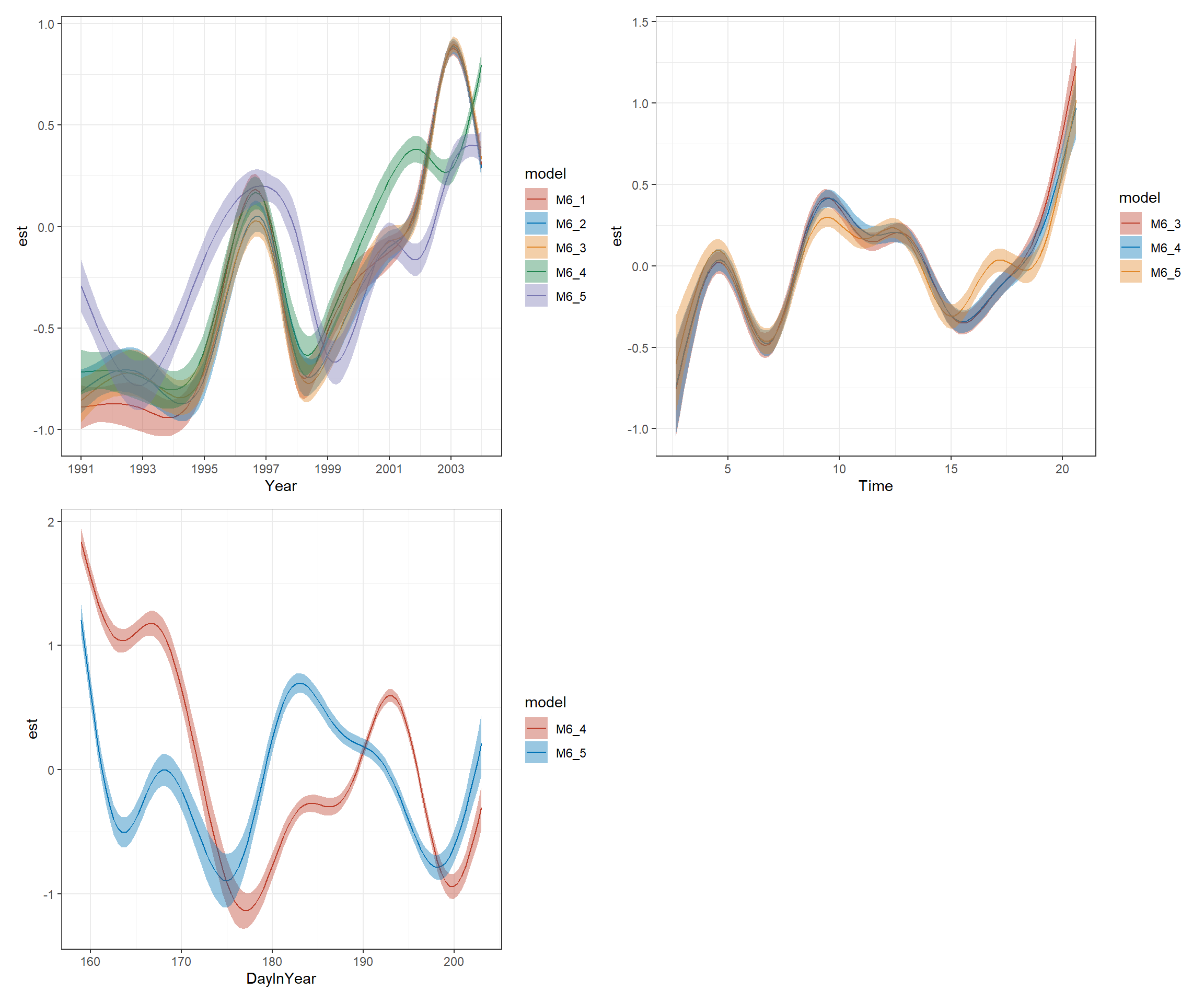
図6.7: Smoothers estimated by GAM
さて、次に以下のような3次元smootherを含めたモデルを考える。
\[
\begin{aligned}
G_i &\sim Poisson(\mu_i)\\
log(\mu_i) &= \alpha + f_1(Times_i) + f_2(DayInYear_i) + f_3(X_i,Y_i, Year_i) + \beta \times Seastate_i + LSA_i \\
\end{aligned}
\]
Rでは以下のように実行する。
M6_6 <- gam(G ~  s(Time) + s(DayInYear) + te(Xkm, Ykm, Year) + offset(LArea) + factor(Seastate),
            family = poisson, data = Gannets2)
このモデルでは、3次元smootherの自由度は123とかなり大きくなる。
##
## Family: poisson
## Link function: log
##
## Formula:
## G ~ s(Time) + s(DayInYear) + te(Xkm, Ykm, Year) + offset(LArea) +
##     factor(Seastate)
##
## Parametric coefficients:
##                   Estimate Std. Error z value Pr(>|z|)
## (Intercept)       -0.51861    0.04676 -11.091  < 2e-16 ***
## factor(Seastate)1  0.01075    0.04488   0.240  0.81060
## factor(Seastate)2 -0.30140    0.04530  -6.653 2.87e-11 ***
## factor(Seastate)3 -0.34641    0.04708  -7.358 1.87e-13 ***
## factor(Seastate)4 -0.56874    0.05160 -11.022  < 2e-16 ***
## factor(Seastate)5 -0.20972    0.06664  -3.147  0.00165 **
## factor(Seastate)6 -0.52544    0.10116  -5.194 2.06e-07 ***
## ---
## Signif. codes:  0 '***' 0.001 '**' 0.01 '*' 0.05 '.' 0.1 ' ' 1
##
## Approximate significance of smooth terms:
##                      edf Ref.df Chi.sq p-value
## s(Time)            8.970      9  428.8  <2e-16 ***
## s(DayInYear)       8.964      9 1028.6  <2e-16 ***
## te(Xkm,Ykm,Year) 123.478    124 8278.1  <2e-16 ***
## ---
## Signif. codes:  0 '***' 0.001 '**' 0.01 '*' 0.05 '.' 0.1 ' ' 1
##
## R-sq.(adj) =  0.0597   Deviance explained = 29.9%
## UBRE = 1.6513 Scale est. = 1 n = 12820分散パラメータ\(\phi\)を計算すると、まだ過分散は解決されていない。
## [1] 12.07028次に、式(6.1)の拡張として、TimeとDayInYearの2次元smootherを考えることもできる。
\[
\begin{aligned}
G_i &\sim Poisson(\mu_i)\\
log(\mu_i) &= \alpha + f_1(Year_i) + f_2(Times_i, DayInYear_i) + f_3(X_i,Y_i) + \beta \times Seastate_i + LSA_i \\
\end{aligned} \tag{6.2}
\]
Rでは以下のように実行する。
M6_7 <- gam(G ~  s(Year) + te(Time, DayInYear) + te(Xkm, Ykm) + offset(LArea) + factor(Seastate),
family = poisson, data = Gannets2)分散パラメータ\(\phi\)を計算すると、まだ過分散は解決されていない。
## [1] 17.8385モデルM6_7の残差と予測値の関係を図示したのが図6.8である。いくつか残差の大きなデータがあることが分かり、図6.6と合わせるとこれらのデータが過分散の原因になっているのではないかと思われる。
data.frame(resid = resid(M6_7, type = "pearson"),
           fitted = fitted(M6_7)) %>%
  ggplot(aes(x = fitted, y = resid))+
  geom_point(shape = 1)+
  theme_bw()+
  theme(aspect.ratio = 1)+
  labs(x = "Fitted values", y = "Pearson residuals")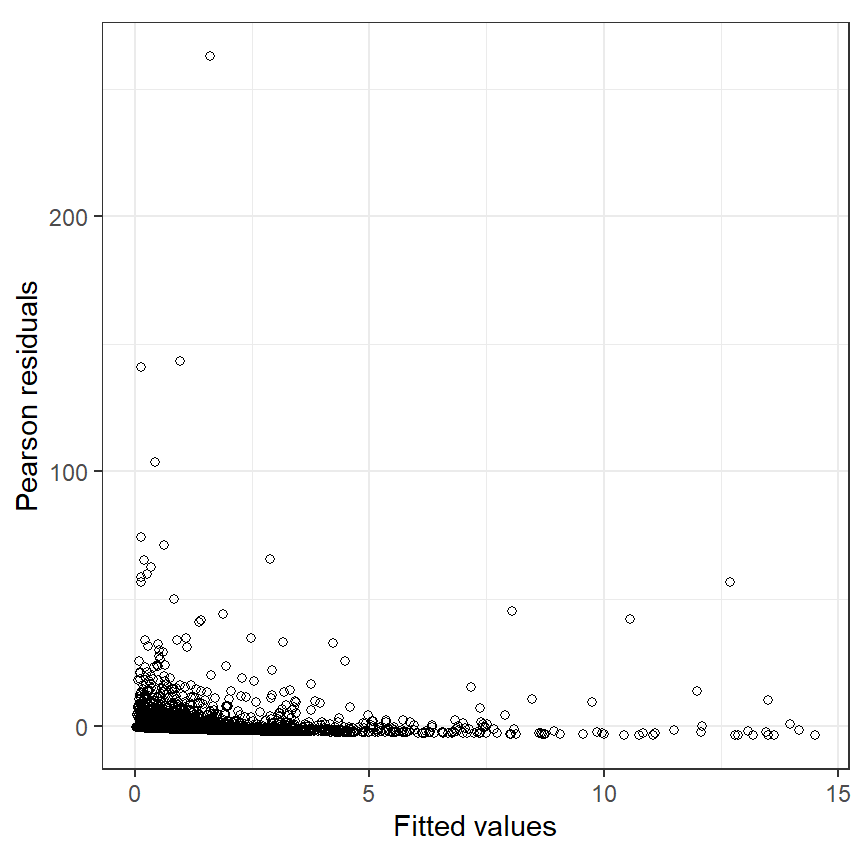
図6.8: Pearson residuals plotted versus fitted values for the Poisson GAM in Equation (6.7).
そのため、次のステップとして自然なのはポワソン分布よりも大きな分散をとりうる負の二項分布を目的変数の分布として仮定することである。
\[ \begin{aligned} G_i &\sim Poisson(\mu_i)\\ E(G_i) &= \mu_i \;\; and \;\;var(G_i) = \mu_i + \frac{\mu_i^2}{k} \\ log(\mu_i) &= \alpha + f_1(Year_i) + f_2(Times_i, DayInYear_i) + f_3(X_i,Y_i) + \beta \times Seastate_i + LSA_i \\ \end{aligned} \tag{6.3} \]
Rではパラメータ\(k\)がthetaとして推定される。以下のように実行できる。
M6_8 <- gam(G ~  s(Year) + te(Time, DayInYear) + te(Xkm, Ykm) + offset(LArea) + factor(Seastate),
family = nb, data = Gannets2)モデルの分散パラメータ\(\phi\)は3.44である。
## [1] 3.441738結果は以下のとおりである。モデルのsmootherは全て有意であり、\(k\)(theta)は0.151と推定された。smootherの自由度はUBRE(unbiased risk estimator)に基づいて推定されている。
##
## Family: Negative Binomial(0.151)
## Link function: log
##
## Formula:
## G ~ s(Year) + te(Time, DayInYear) + te(Xkm, Ykm) + offset(LArea) +
##     factor(Seastate)
##
## Parametric coefficients:
##                   Estimate Std. Error z value Pr(>|z|)
## (Intercept)       -0.42313    0.10208   -4.15  3.4e-05 ***
## factor(Seastate)1  0.35118    0.12656    2.77   0.0055 **
## factor(Seastate)2 -0.10057    0.11859   -0.85   0.3964
## factor(Seastate)3 -0.00582    0.11539   -0.05   0.9597
## factor(Seastate)4 -0.26035    0.12001   -2.17   0.0301 *
## factor(Seastate)5 -0.12681    0.14264   -0.89   0.3740
## factor(Seastate)6 -0.41042    0.18740   -2.19   0.0285 *
## ---
## Signif. codes:  0 '***' 0.001 '**' 0.01 '*' 0.05 '.' 0.1 ' ' 1
##
## Approximate significance of smooth terms:
##                      edf Ref.df Chi.sq p-value
## s(Year)             6.79   7.83   99.1  <2e-16 ***
## te(Time,DayInYear) 20.43  22.58  167.3  <2e-16 ***
## te(Xkm,Ykm)        15.40  17.93  517.8  <2e-16 ***
## ---
## Signif. codes:  0 '***' 0.001 '**' 0.01 '*' 0.05 '.' 0.1 ' ' 1
##
## R-sq.(adj) =  0.0259   Deviance explained = 23.6%
## -REML = 10345 Scale est. = 1 n = 12820残差と予測値の関係を図示したのが図6.8である。赤い点はカツオドリの数が25以上のポイントである。この図から、モデルはカツオドリの数が大きいポイントをうまくフィットできていないことが示唆される。
data.frame(resid = resid(M6_8, type = "pearson"),
           fitted = fitted(M6_8),
           G = Gannets2$G) %>%
  ggplot(aes(x = fitted, y = resid))+
  geom_point(shape = 1,
             aes(color = G >= 25),
             stroke = 1.1,
             alpha = 0.3)+
  theme_bw()+
  theme(aspect.ratio = 1)+
  labs(x = "Fitted values", y = "Pearson residuals")+
  scale_color_manual(values = c("black", "red3"))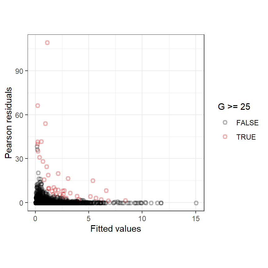
図6.9: Pearson residuals plotted versus fitted values for the negative binomial GAM in Equation (6.8). The values plotted with a red dot are observations for which the gannet abundance exceeds 25.
また、残差に空間的な相関がないかを確かめるため、ピアソン残差を利用したバリオグラムを描いたのが図6.10である。図からは、深刻な空間的相関があるようには見えない。
mydata <- data.frame(resid = resid(M6_8, type = "pearson"),
                     Xkm = Gannets2$Xkm,
                     Ykm = Gannets2$Ykm)

sp::coordinates(mydata) <- c("Xkm","Ykm")

Vario_M6_8 <- variogram(resid ~ 1, mydata, cutoff = 5, robust = TRUE)

Vario_M6_8 %>%
  ggplot(aes(x = dist, y = gamma))+
  geom_point(aes(size = np))+
  theme_bw()+
  theme(aspect.ratio = 1)+
  labs(y = "Semi-variogram", x = "Distance (km)")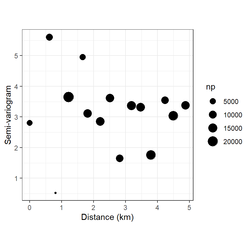
図6.10: Sample variogram of Pearson residuals from the negative binomial GAM. Point size is proportional to the number of combinations of sites used for calculating the sample variogram at a particular distance.
推定されたte(DayInYear, Time)のsmootherは以下のとおりである(図6.11。解釈は難しいが、日付や時刻によってばらつきがかなりあることが分かる。
smooth_estimates(M6_8, smooth = "te(Time,DayInYear)") %>%
  plot_ly() %>%
  add_trace(x = ~DayInYear,
          y = ~Time,
          z = ~est,
          type = "mesh3d")
図6.11: Estimated sm oothers te(DayInYear, TimeH) for the negative binomial GAM.
推定されたte(Xkm, Ykm)のsmootherは以下のとおりである図6.12)。こちらは、南西のエリアでカツオドリがよく目撃されていることを示している。
smooth_estimates(M6_8, smooth = "te(Xkm,Ykm)") %>%
  plot_ly() %>%
  add_trace(x = ~Xkm,
          y = ~Ykm,
          z = ~est,
          type = "mesh3d")
図6.12: Estimated smoot hers te(Xkm, Ykm) for the negative binomial GAM.
観察年(Year)のsmootherは図6.13の通り。カツオドリの数は1993年から1997年ごろにかけて急増し、その後減少したが2000年ごろからもう一度増加するというパターンをとっていた。
smooth_estimates(M6_8, smooth = "s(Year)") %>%
  add_confint() %>%
  ggplot(aes(x = Year, y = est))+
  geom_line()+
  geom_ribbon(aes(ymin = lower_ci, ymax = upper_ci),
              alpha = 0, linetype = "dashed", color = "black")+
  theme_bw()+
  theme(aspect.ratio = 1)+
  scale_x_continuous(breaks = seq(1991,2006,by=2))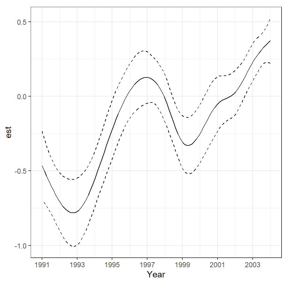
図6.13: Estimated smoothers s(Y ear) for the negative binomial GAM.
6.6 Zero-inflated GAM
前節で適用した負の二項分布モデルは依然として過分散であった。過分散には様々な原因があるが、 Zuur et al. (2012) は外れ値、必要な共変量が入っていない、交互作用がひっていない、リンク関数が誤っている、目的変数のばらつきが大きすぎる、時空間的な相関がモデルで考慮されていない、ゼロ過剰などが過分散の要因の大部分を占めると論じている。
空間的な相関とゼロ過剰はしばしば交絡しやすい(隣のトランゼクトが0を持つ確率が高くなるなど)[Zuur2012b]。そのため、空間的な構造を考慮したGAMをモデリングすることも可能である(e.g., CARモデルなど)。一方で、ゼロ過剰モデルを作ることも可能である。両方を適用すると問題が生じることが多いので、生物学的な知識に基づいてどちらを適用すべきか決める必要がある。
空間的な相関を取り入れるモデルはベイズ統計を必要とし、本稿の範囲を超えるので今回はゼロ過剰モデルを適用する。
6.6.1 A zero-inflated model for the gannet data
ゼロ過剰モデルにはいくつかの種類があるが、ここではいわゆる混合モデル(mixture model)を適用する。混合モデルは偽物のゼロと真のゼロを区別する。偽物のゼロは、サンプリングが間違ったときに行われた(e.g., カツオドリがいない冬に観察を行った)、観察エラー(e.g., 天候などで視界が悪い)、動物のエラー(e.g., カツオドリがいるはずだがいなかった)などのときに生じる。真のゼロはそうした要因以外に動物がいないときに生じる。
混合ゼロ過剰モデルでは2つのGLM(またはGAM)がくっつけられている。真のゼロとゼロより大きい値に対して適用するポワソンまたは負の二項GLM(GAM)とそれでは説明できない偽物のゼロに対して適用される二項分布モデルである。詳しくはこちらや Zuur et al. (2012) も参照。
混合ゼロ過剰モデルでは、まず偽物のゼロが得られる確率\(\pi_i\)を二項分布モデルでモデリングする。ここでは、\(\pi_i\)が一つのパラメータ\(\gamma\)のみで決まると仮定しているが、様々な共変量によって変化するとモデリングすることも可能である(e.g., \(logit(\pi_i) = \gamma_0 + \gamma_1 \times Seastate_i + f_\gamma(Year)\))。これは、生物学的知識に基づいて行われる必要がある。
\[ \begin{aligned} logit(\pi_i) &= \gamma\\ \end{aligned} \]
そのうえで、ゼロ過剰モデルでは偽物のゼロ以外(真のゼロと0より大きい値)についてポワソン分布または負の二項分布を適用する。例えばポワソン分布を適用するとき、平均\(\mu_i\)のポワソン分布で値\(Y_i\)をとる確率は\(P(Y_i|\mu_i) = \frac{\mu_i^{Y_i} \times r^{-\mu_i}}{Y_i!}\)なので、真のゼロが得られる確率は以下のようになる。
\[ \frac{\mu_i^0 \times e^{-\mu_i}}{0!} = e^{-\mu_i} \]
よって、ゼロ過剰モデルでゼロ(偽物+真)が得られる確率は、偽物のゼロ以外が得られる確率が\(1-\pi_i\)であることを考えると以下のようになる。
\[ \pi_i + (1-\pi_i) \times e^{-\mu_i} \]
ゼロ以外の値についてはポワソン分布や負の二項分布が通常通り適用される。合わせると、ゼロ過剰ポワソンGAMのモデル式は以下のように書ける。なお、\(G_i \sim ZIP(\mu_i, \pi_i)\)はポワソン分布の平均が\(\mu_i\)、偽物のゼロが得られる確率が\(\pi_i\)の混合モデルからカツオドリの数が得られることを指す。
\[ \begin{aligned} G_i &\sim ZIP(\mu_i, \pi_i)\\ log(\mu_i) &= \alpha + f_1(Year_i) + f_2(Times_i, DayInYear_i) + f_3(X_i,Y_i) + \beta \times Seastate_i + LSA_i \\ logit(\pi_i) &= \gamma\\ E(G_i) &= (1-\pi_i) \times \mu_i \;\; and \;\;var(G_i) = (1-\pi_i) \times(\mu_i + \pi_i \times \mu_i)\\ \end{aligned} \tag{6.4} \]
ゼロ過剰GAMを実行できるRパッケージはCOZIGAM、VGAM、gamlssなどがあるが、本章ではgamlssパッケージを用いて実行する。
⇒ 現在ではmgvcパッケージでもゼロ過剰ポワソン分布がサポートされているが、リンク関数は恒等関数しかないよう。
6.6.2 ZIP GAM using gamlss
2次元smootherを導入するためには、gamlssのヘルパーパッケージであるgamlss.addも読み込む必要がある。以下、式(6.4)のモデル式をRで実行したものである。gamlssではmgcvのように交差検証による自由度の選択は行ってくれず、使用者が上限を指定する必要がある。以下のモデルでは、M6_8の結果をもとに自由度を\(k =\)で指定している。2次元smootherはga(~te(Time, DayInYear))のように式に加える。座標の2次元smootherはte(Xkm,Ykm)とするとエラーが出て実行できなかったので、s(Xkm,Ykm)。これらの変数は異なるスケールを持つため、前述したようにこれは問題になりうる。
モデルは収束せず…。
## iterationの数を設定
con <- gamlss.control(n.cyc = 200)

#M6_9 <- gamlss(G ~ cs(Year, df = 8) + ga(~te(Time, DayInYear, fx = TRUE, k = 28)) +
 #               ga(~s(Xkm,Ykm, fx = TRUE, k=28)) + factor(Seastate) + offset(LArea),
# family = ZIP(), data = Gannets2, control = con)ベイズモデリングでの実装はbrmsパッケージでできる。brmsではテンソル積smootherとしてte()は実装していないが、代わりにt2()が使える。詳しくはこちら。
以下のように実行できる。こちらもかなり長い時間を要する。
## 高速化オプション
rstan_options(auto_write = TRUE)
options(mc.cores = parallel::detectCores())

M6_9 <- brm(G ~  s(Year) + t2(Time, DayInYear) + t2(Xkm, Ykm) + offset(LArea) + factor(Seastate),
            family = "zero_inflated_poisson", data = Gannets2,
            backend = "cmdstanr",
            control=list(adapt_delta = 0.99, max_treedepth = 15),
file = "result/M6_9")結果は以下の通り。Population Effect Levelとして推定されているのは回帰係数のようだ。sdsの部分はsmootherの自由度のようなものを推定しているよう。詳しい見方は不明である。偽物のゼロが得られる確率(zi)は0.75と推定された。
##  Family: zero_inflated_poisson
##   Links: mu = log; zi = identity
## Formula: G ~ s(Year) + t2(Time, DayInYear) + t2(Xkm, Ykm) + offset(LArea) + factor(Seastate)
##    Data: Gannets2 (Number of observations: 12820)
##   Draws: 4 chains, each with iter = 2000; warmup = 1000; thin = 1;
##          total post-warmup draws = 4000
##
## Smooth Terms:
##                        Estimate Est.Error l-95% CI u-95% CI Rhat Bulk_ESS
## sds(sYear_1)              13.19      3.51     7.66    21.21 1.00     1338
## sds(t2TimeDayInYear_1)    34.80      8.09    22.89    54.08 1.00     1164
## sds(t2TimeDayInYear_2)    16.93      4.66    10.43    28.85 1.00     1749
## sds(t2TimeDayInYear_3)    10.91      3.31     6.29    18.58 1.00     1835
## sds(t2XkmYkm_1)           10.72      2.92     6.43    17.95 1.00     1592
## sds(t2XkmYkm_2)           10.27      3.03     6.23    17.55 1.00     1807
## sds(t2XkmYkm_3)            1.30      1.11     0.05     4.18 1.00     1473
##                        Tail_ESS
## sds(sYear_1)               1959
## sds(t2TimeDayInYear_1)     1567
## sds(t2TimeDayInYear_2)     2149
## sds(t2TimeDayInYear_3)     2069
## sds(t2XkmYkm_1)            1986
## sds(t2XkmYkm_2)            2297
## sds(t2XkmYkm_3)            2375
##
## Population-Level Effects:
##                   Estimate Est.Error l-95% CI u-95% CI Rhat Bulk_ESS Tail_ESS
## Intercept             1.14      0.09     0.97     1.31 1.00     2258     2668
## factorSeastate1       0.01      0.05    -0.08     0.10 1.00     3162     2939
## factorSeastate2      -0.12      0.05    -0.21    -0.03 1.00     3345     3108
## factorSeastate3      -0.33      0.05    -0.42    -0.23 1.00     2941     2916
## factorSeastate4      -0.54      0.05    -0.64    -0.44 1.00     3047     3143
## factorSeastate5      -0.57      0.06    -0.70    -0.45 1.00     3820     3365
## factorSeastate6      -1.03      0.11    -1.25    -0.82 1.00     5619     3356
## sYear_1               2.66      2.94    -3.00     8.29 1.00     5011     3299
## t2TimeDayInYear_1    -0.07      0.04    -0.14     0.00 1.00     2325     2198
## t2TimeDayInYear_2    -0.08      0.05    -0.17     0.01 1.00     1744     2530
## t2TimeDayInYear_3     0.03      0.03    -0.04     0.09 1.00     1836     2197
## t2XkmYkm_1            0.07      0.07    -0.07     0.20 1.00     2480     2339
## t2XkmYkm_2           -0.32      0.06    -0.45    -0.21 1.00     1938     1917
## t2XkmYkm_3           -0.09      0.10    -0.27     0.11 1.00     2066     1708
##
## Family Specific Parameters:
##    Estimate Est.Error l-95% CI u-95% CI Rhat Bulk_ESS Tail_ESS
## zi     0.75      0.00     0.74     0.76 1.00     6762     2642
##
## Draws were sampled using sample(hmc). For each parameter, Bulk_ESS
## and Tail_ESS are effective sample size measures, and Rhat is the potential
## scale reduction factor on split chains (at convergence, Rhat = 1).DHARMaパッケージを用いて過分散の検定を行うことができる。その結果、過分散はまだ解消されていないようだ。
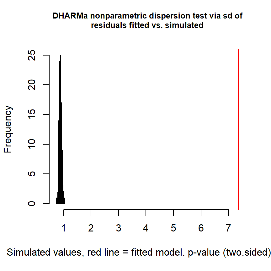
##
##  DHARMa nonparametric dispersion test via sd of residuals fitted vs.
##  simulated
##
## data:  simulationOutput
## dispersion = 8.3151, p-value < 2.2e-16
## alternative hypothesis: two.sided次のオプションとして、ゼロ過剰負の二項分布のGAMを用いることができる。brmsのみで実装できるようだ。こちらも長い時間を要する。
Gannets2 <- Gannets2 %>% mutate(fSeastate = factor(Seastate))

M6_10 <- brm(G ~  s(Year) + t2(Time, DayInYear) + t2(Xkm, Ykm) + offset(LArea) + fSeastate,
            family = "zero_inflated_negbinomial", data = Gannets2,
            backend = "cmdstanr",
            control=list(adapt_delta = 0.99, max_treedepth = 15),
            file = "result/M6_10")
結果は以下の通り。偽物のゼロが得られる確率はほとんどない(0.01)と推定されている。
##  Family: zero_inflated_negbinomial
##   Links: mu = log; shape = identity; zi = identity
## Formula: G ~ s(Year) + t2(Time, DayInYear) + t2(Xkm, Ykm) + offset(LArea) + fSeastate
##    Data: Gannets2 (Number of observations: 12820)
##   Draws: 4 chains, each with iter = 2000; warmup = 1000; thin = 1;
##          total post-warmup draws = 4000
##
## Smooth Terms:
##                        Estimate Est.Error l-95% CI u-95% CI Rhat Bulk_ESS
## sds(sYear_1)               5.85      2.33     2.54    11.59 1.00     1156
## sds(t2TimeDayInYear_1)     2.78      1.78     0.68     7.21 1.00      990
## sds(t2TimeDayInYear_2)     7.55      2.77     3.73    14.43 1.00     1492
## sds(t2TimeDayInYear_3)     1.58      1.16     0.07     4.36 1.00     1174
## sds(t2XkmYkm_1)            1.56      1.25     0.06     4.62 1.01     1062
## sds(t2XkmYkm_2)            7.10      2.29     3.65    12.57 1.00     1456
## sds(t2XkmYkm_3)            4.00      1.88     0.88     8.37 1.00      924
##                        Tail_ESS
## sds(sYear_1)               2206
## sds(t2TimeDayInYear_1)     1679
## sds(t2TimeDayInYear_2)     1711
## sds(t2TimeDayInYear_3)     1515
## sds(t2XkmYkm_1)            1911
## sds(t2XkmYkm_2)            2343
## sds(t2XkmYkm_3)             710
##
## Population-Level Effects:
##                   Estimate Est.Error l-95% CI u-95% CI Rhat Bulk_ESS Tail_ESS
## Intercept            -0.63      0.16    -0.93    -0.31 1.00     1092     1825
## fSeastate1            0.37      0.13     0.10     0.62 1.00     1707     2531
## fSeastate2           -0.13      0.12    -0.38     0.10 1.00     1625     2650
## fSeastate3           -0.03      0.12    -0.27     0.19 1.00     1555     2198
## fSeastate4           -0.31      0.12    -0.56    -0.07 1.00     1602     2554
## fSeastate5           -0.13      0.15    -0.43     0.16 1.00     1905     2726
## fSeastate6           -0.45      0.20    -0.84    -0.06 1.00     2623     3123
## sYear_1              -1.79      4.36   -10.67     6.57 1.00     2574     2470
## t2TimeDayInYear_1    -0.29      0.06    -0.40    -0.18 1.00     1879     2447
## t2TimeDayInYear_2    -0.04      0.06    -0.16     0.08 1.00     2452     2694
## t2TimeDayInYear_3    -0.08      0.05    -0.17     0.03 1.00     2185     2875
## t2XkmYkm_1            0.30      0.13     0.06     0.56 1.00      934     1512
## t2XkmYkm_2           -0.52      0.11    -0.73    -0.31 1.00      832     1165
## t2XkmYkm_3           -0.35      0.18    -0.73    -0.01 1.00      869     1402
##
## Family Specific Parameters:
##       Estimate Est.Error l-95% CI u-95% CI Rhat Bulk_ESS Tail_ESS
## shape     0.15      0.00     0.14     0.16 1.00     5725     3006
## zi        0.01      0.01     0.00     0.03 1.00     3312     2424
##
## Draws were sampled using sample(hmc). For each parameter, Bulk_ESS
## and Tail_ESS are effective sample size measures, and Rhat is the potential
## scale reduction factor on split chains (at convergence, Rhat = 1).DHARMaパッケージを用いて過分散の検定を行うことができる。過分散はかなり改善されたがまだ少し残っているようだ。
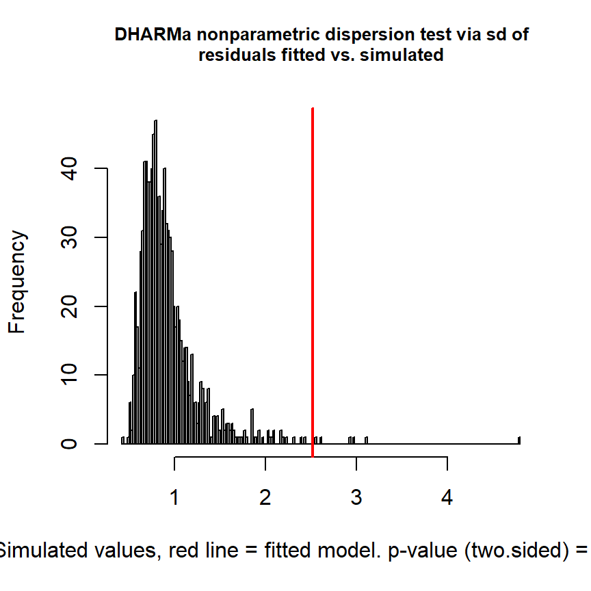
##
##  DHARMa nonparametric dispersion test via sd of residuals fitted vs.
##  simulated
##
## data:  simulationOutput
## dispersion = 2.7193, p-value = 0.012
## alternative hypothesis: two.sided年のsmoother(s(Year))の推定結果は以下のようになる(図6.14)。M6_8とほとんど変わらない。
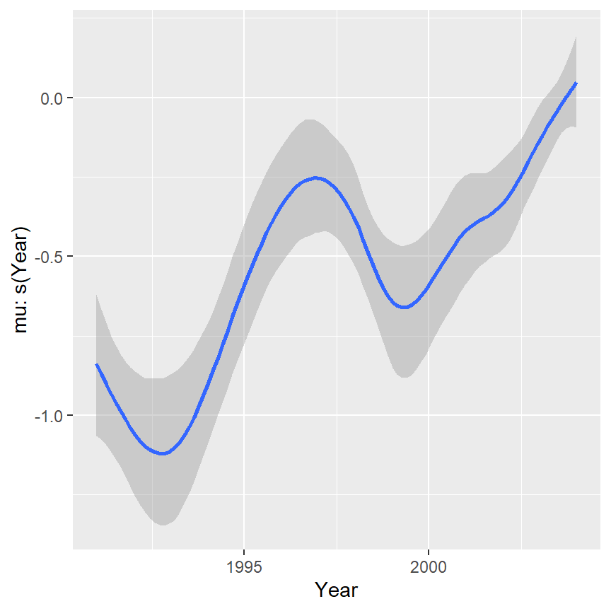
図6.14: Estimated smoother of s(Year) based on M6_10
緯度と経度の2次元smoother(t2(Xkm,Ykm))の推定結果は以下のようになる(図6.15)。
conditional_effects(M6_10, effects = "Xkm:Ykm")[[1]] %>%
  plot_ly() %>%
  add_trace(x = ~Xkm,
          y = ~Ykm,
          z = ~estimate__,
          type = "mesh3d")
図6.15: Estimated smoother of t2(Xkm,Ykm) based on M6_10
最後に、時刻と日付の2次元smoother(t2(Time,DayInYear))の推定結果は以下のようになる(図6.15)。
conditional_effects(M6_10, effects = "Time:DayInYear")[[1]] %>%
  plot_ly() %>%
  add_trace(x = ~Time,
          y = ~DayInYear,
          z = ~estimate__,
          type = "mesh3d")
図6.16: Estimated smoother of t2(Time,DayInYear) based on M6_10