2 Introduction to additive models using deep-sea fisheries data
本章では、正規分布に従う一般化加法モデル(GAM)の導入を行う。
2.1 Impact of deep-sea fisheries
本章では、商業的な漁業が深海(水深800–4865m)の魚の密度に及ぼす影響を調べた Bailey et al. (2009) のデータを用いる。データは2つの期間に分かれており、1979年から1989年は商業的な漁業がおこなわれる前(深い水深での漁業が発展している段階)で、1997年から2002年は商業的漁業がおこなわれている時期である。商業的漁業は技術的または商業的な理由により水深約1600mまでに限られている。
fish <- read_delim("data/BaileyDensity.txt")

datatable(fish,
          options = list(scrollX = 20),
filter = "top")期間ごとにデータをサンプリングした場所を示したのが図2.1である。Periodは1が1979–1989年を、2が1997–2002年を表す。
fish %>%
  mutate(Period = as.factor(Period)) %>%
  ggplot(aes(x = Xkm, y = Ykm))+
  geom_point(aes(fill = Period),
             shape = 21, alpha = 0.6)+
  theme_bw()+
  theme(aspect.ratio = 1)+
  scale_fill_manual(values = c("white","black"))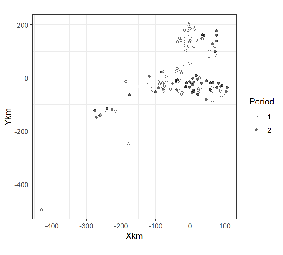
図2.1: Position of the Sites
Bailey et al. (2009) では、魚の密度を以下のように定義している。
\[ 場所iにおける魚の密度 = \frac{場所iの魚の総量}{場所iで探索を行った面積} \]
密度のような割り算データを目的変数にして正規分布に当てはめると、等分散性の問題が生じることが多い。通常、このような分子が整数値の割り算データに対してはポワソン分布や負の二項分布でオフセット項を用いる(第4章を参照)。もし分母が試行数、分子が成功数などのカウントデータの場合は二項分布を当てはめた方がよい。密度が0より大きい値しかとらないのであれば、ガンマ分布を当てはめることもできる。
2.2 First encounter with smoothers
2.2.1 Applying linear regression
2.2.1.1 当てはめるモデル
全種を含めた魚の密度は以下のように表せる。なお\(i\)は場所を、\(j\)は魚の種類を表す。また、\(SA_i\)は場所\(i\)における探索面積を、\(Y_{ij}\)は場所\(i\)における種\(j\)の捕獲個体数を表す。 \[ Dens_i = \frac{\sum_j Y_{ij}}{SA_i} \]
まずは、各探索場所の深さのみが魚の密度に影響するとする線形なモデルを考える。モデル式は以下のようになる。
\[ \begin{aligned} Dens_i &= \alpha + \beta \times Depth_i + \epsilon_i \\ \epsilon_i &\sim N(0,\sigma^2) \end{aligned} \]
2.2.1.2 data exploration
いかなるモデルを作ろうとも、まずはデータ探索を行う。まずは、水深と魚の密度の関連をプロットする(図2.2)。図から明らかに水深と魚の密度の関係は線形ではない。しかし、ここではこうしたデータが線形モデルの前提を満たさないことを示すため、まずは通常の線形モデルを適用する。
fish %>%
  filter(MeanDepth > 800) %>%
  mutate(year01 = ifelse(Year > 1990, "commercial","non-commercial")) %>%
  ggplot(aes(x = MeanDepth, y = Dens))+
  geom_point(aes(shape = year01))+
  scale_shape_manual(values = c(19,1)) +
  theme_bw()+
  theme(aspect.ratio = 1,
        legend.position = "none")+
  labs(x = "Mean sampling depth (m)",
       y = expression(paste("Fish density"," ", (m^2))))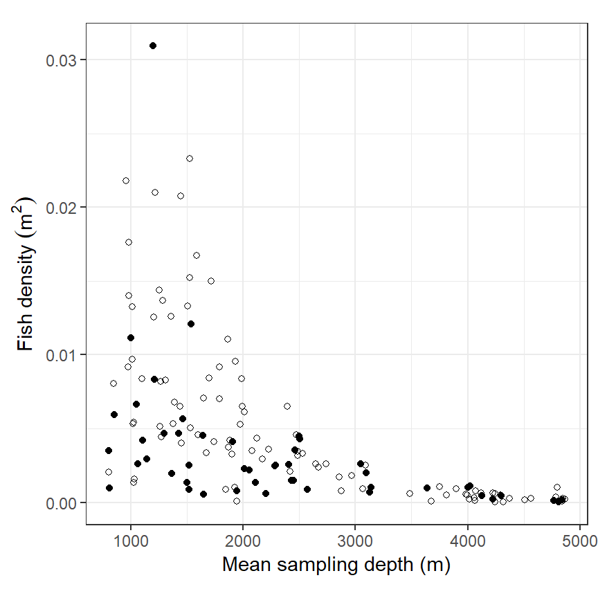
図2.2: Relationship between fish density and mean sampling depth. Filled circles are observations from the second period and open circles from the first period.
モデルは以下のように実行できる。モデルは、目的変数のばらつきの33.7%が水深で説明できると推定している(Adjusted R-squaredより)。
fish %>%
  filter(MeanDepth > 800) %>%
  na.omit() -> fish

M2_1 <- lm(Dens ~ MeanDepth, data = fish)

print(summary(M2_1), digits = 3)
##
## Call:
## lm(formula = Dens ~ MeanDepth, data = fish)
##
## Residuals:
## Min 1Q Median 3Q Max
## -0.007835 -0.002519 -0.000558 0.001420 0.023109
##
## Coefficients:
## Estimate Std. Error t value Pr(>|t|)
## (Intercept) 1.09e-02 8.06e-04 13.51 <2e-16 ***
## MeanDepth -2.56e-06 2.96e-07 -8.63 1e-14 ***
## ---
## Signif. codes: 0 '***' 0.001 '**' 0.01 '*' 0.05 '.' 0.1 ' ' 1
##
## Residual standard error: 0.00449 on 145 degrees of freedom
## Multiple R-squared: 0.339, Adjusted R-squared: 0.335
## F-statistic: 74.4 on 1 and 145 DF, p-value: 1.02e-142.2.1.3 model diagnosis
それでは、モデル診断を行おう。
まずは標準化残差とモデルの予測値の関係を見る(図2.3のA)。明らかにパターンが見て取れ、モデルが等分散性の仮定を満たしていないことが分かる。また、水深と標準化残差にもパターンがあるように見え(図2.3のB)、このモデルでは水深でうまく目的変数を説明できていないことが分かる。
data.frame(resstd = rstandard(M2_1),
           fitted = fitted(M2_1)) %>%
  ggplot(aes(x = fitted, y = resstd))+
  geom_point()+
  geom_hline(yintercept = 0)+
  theme_bw()+
  theme(aspect.ratio = 1)+
  labs(x = "Fitted values", y = "Standardized residuals",
       title = "A") -> p_diag_M2_1_a

data.frame(resstd = rstandard(M2_1),
           depth = fish$MeanDepth) %>%
  ggplot(aes(x = depth, y = resstd))+
  geom_point()+
  geom_hline(yintercept = 0)+
  theme_bw()+
  theme(aspect.ratio = 1)+
  labs(x = "Mean Depth", y = "Standardized residuals",
       title = "B") -> p_diag_M2_1_b

p_diag_M2_1_a + p_diag_M2_1_b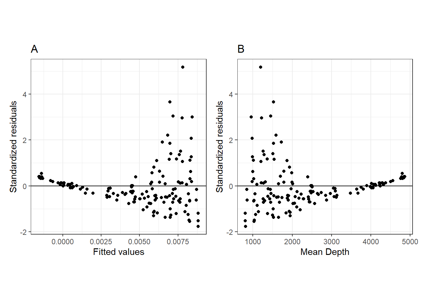
図2.3: A. Standardized residuals versus fitted values to assess homogeneity. B. Residuals versus mean depth.
QQプロットでも標準化残差が標準正規分布に従っていないことが示唆される。
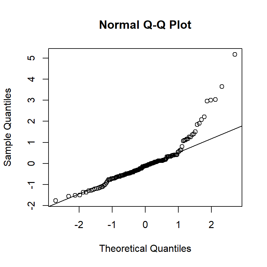
図2.4: QQplot for M2_1
残差に見られたパターンは、明らかに非線形なデータに直線的なモデルを当てはめているために生じている。図2.5からわかるように、水深2000m以上ではモデルに基づく回帰直線がほとんどデータの上に来てしまっている。また、水深約4000m以上では予測値がマイナスになってしまっている。
dataM2_1 <- data.frame(MeanDepth = seq(800,5000,length.out = 100))

pred_M2_1 <- predict(M2_1,
                    newdata = dataM2_1) %>%
  data.frame() %>%
  rename(pred = 1) %>%
  bind_cols(dataM2_1)

pred_M2_1 %>%
  ggplot(aes(x = MeanDepth, y = pred))+
  geom_line()+
  geom_point(data = fish,
             aes(y = Dens))+
  theme_bw()+
  theme(aspect.ratio = 1)+
  labs(x = "Mean Depth", y = expression(paste("Fish density"," ", (m^2))))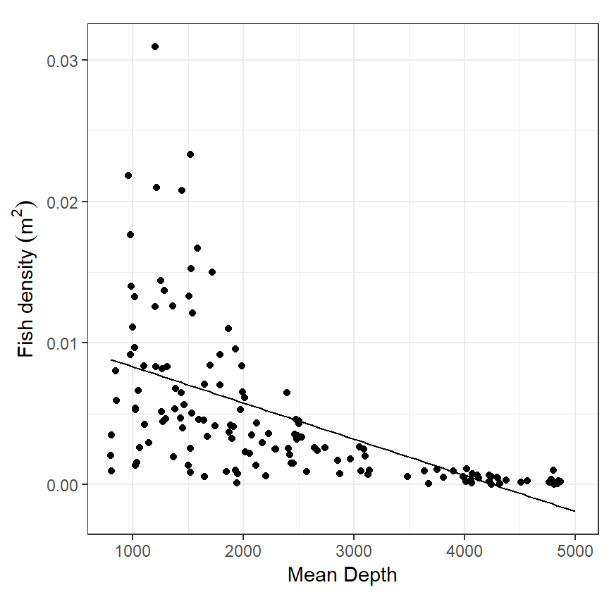
図2.5: Fidh density plotted versus depth, with fitted values obtained by linear model.
2.2.2 Applying cubic polynomials
モデルを改善するため、説明変数に水深の二乗、三乗、四乗項を入れるモデルを考える(= 多項式回帰)。このようにすることで非線形な関係をとらえられるかもしれない。
\[ \begin{aligned} Dens_i &= \alpha + \beta_1 \times Depth_i + \beta_2 \times Depth^2_i + \beta_3 \times Depth^3_i + \epsilon_i \\ \epsilon_i &\sim N(0,\sigma^2) \end{aligned} \]
そのようなモデルは以下で実行できる。
モデルの診断を行ったのが図2.6である。明確なパターンがあるように見え(A. 予測値が大きいほどばらつきが大きくなる、B. 水深が浅くなるほどばらつきが大きくなる)、モデルが十分に改善できていないことが分かる。
data.frame(resstd = rstandard(M2_2),
           fitted = fitted(M2_2)) %>%
  ggplot(aes(x = fitted, y = resstd))+
  geom_point()+
  geom_hline(yintercept = 0)+
  theme_bw()+
  theme(aspect.ratio = 1)+
  labs(x = "Fitted values", y = "Standardized residuals",
       title = "A") -> p_diag_M2_2_a

data.frame(resstd = rstandard(M2_2),
           depth = fish$MeanDepth) %>%
  ggplot(aes(x = depth, y = resstd))+
  geom_point()+
  geom_hline(yintercept = 0)+
  theme_bw()+
  theme(aspect.ratio = 1)+
  labs(x = "Mean Depth", y = "Standardized residuals",
       title = "B") -> p_diag_M2_2_b

p_diag_M2_2_a + p_diag_M2_2_b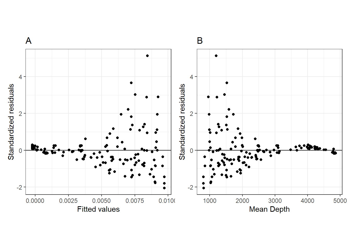
図2.6: A. Standardized residuals versus fitted values to assess homogeneity. B. Residuals versus mean depth.
QQプロットからも標準化残差が標準正規分布に従っていないことが分かる(図2.7)。
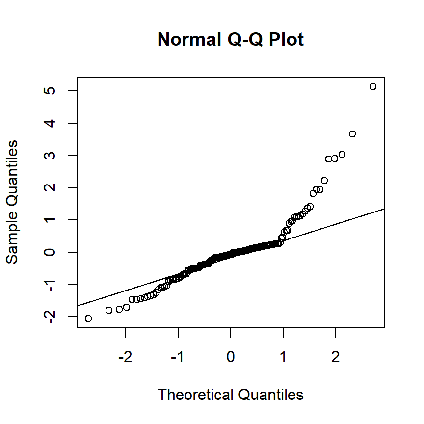
図2.7: QQplot for M2_2
実測値にモデルに基づく予測値を描いたのが図2.8である。水深4000mあたりで予測値がほとんどの実測値よりも低くなってしまっている。
dataM2_2 <- data.frame(MeanDepth = seq(800,5000,length.out = 100))

pred_M2_2 <- predict(M2_2,
                    newdata = dataM2_2) %>%
  data.frame() %>%
  rename(pred = 1) %>%
  bind_cols(dataM2_2)

pred_M2_2 %>%
  ggplot(aes(x = MeanDepth, y = pred))+
  geom_line()+
  geom_point(data = fish,
             aes(y = Dens))+
  theme_bw()+
  theme(aspect.ratio = 1)+
  labs(x = "Mean Depth", y = expression(paste("Fish density"," ", (m^2))))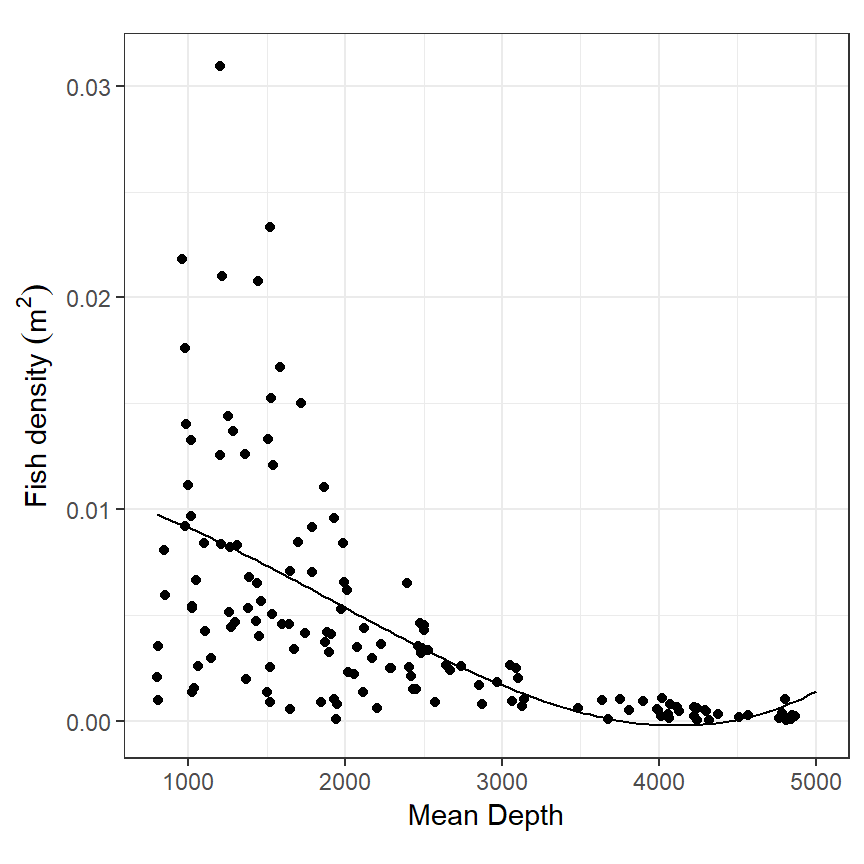
図2.8: Fidh density plotted versus depth, with fitted values obtained by linear model.
2.2.3 A simple GAM
モデルを改善するほかの選択肢は、一般化加法モデル(GAM)を用いることである。シンプルなGAMは以下のように書ける。\(f(Depth_i)\)は平滑化関数であり、予測値がデータに合うような曲線を描くように推定される。以下では、GAMではどのようにしてこの関数を推定するのかを説明していく。
\[ \begin{aligned} Dens_i &= \alpha + f(Depth_i) + \epsilon_i \\ \epsilon_i &\sim N(0,\sigma^2) \end{aligned} \tag{2.1} \]
2.2.4 Moving average and LOESS smoother
データに合うように平滑化を行う方法は複数存在するが、比較的単純なものが移動平均とLOESS(局所回帰)である。より複雑な手法については第3方で解説する。
2.2.4.1 移動平均
移動平均は、推定値を求めたいポイントの前後にある特定の範囲(あるいは個数?)のデータの平均値を推定値とするような方法である。例えば、水深2500mのときの推定値として、その前後500m(2000m ~ 3000m)にあるデータの平均値を用いると、0.00286になる(図2.9)。
fish %>%
  filter(MeanDepth >= 2000 & MeanDepth <= 3000) %>%
  summarise(mean = mean(Dens)) -> mean

fish %>%
  ggplot(aes(x = MeanDepth, y = Dens))+
  geom_point(shape = 1)+
  geom_vline(xintercept = 2000,
             linetype = "dashed")+
  geom_vline(xintercept = 3000,
             linetype = "dashed")+
  geom_point(aes(x = 2500, y = mean$mean),
             size = 5, shape = 18, color = "black")+
  annotate(geom = "text",
           x = 3000, y = mean$mean + 0.002,
           label = sprintf("%.5f",mean$mean))+
  geom_segment(aes(x = 2550, xend = 2900, y = mean$mean, yend = mean$mean + 0.0015))+
  theme_bw()+
  theme(aspect.ratio = 1)+
  labs(x = "Mean Depth", y = expression(paste("Fish density"," ", (m^2))))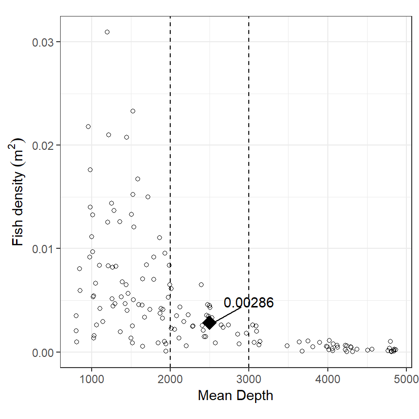
図2.9: Visualization of the process of the moving average. A target value of depth = 2500 was chosen.
これを一定間隔のデータで行ってつなげると、移動平均に基づいて平滑化曲線を描くことができる(図2.10)。
Depth_n <- seq(810, 4800, length.out = 150)
Mean_n <- data.frame(MeanDepth = Depth_n,
                     Est = NA)

for(i in seq_along(Depth_n)){
  fish %>%
    filter(MeanDepth >= Depth_n[i] - 500 & MeanDepth <= Depth_n[i] + 500) %>%
    summarise(mean = mean(Dens)) -> mean_i

  Mean_n[i,2] <- mean_i$mean
}

fish %>%
  ggplot(aes(x = MeanDepth, y = Dens))+
  geom_point(shape = 1)+
  geom_line(data = Mean_n,
            aes(y = Est),
            linewidth = 1)+
  theme_bw()+
  theme(aspect.ratio = 1)+
  labs(x = "Mean Depth", y = expression(paste("Fish density"," ", (m^2))))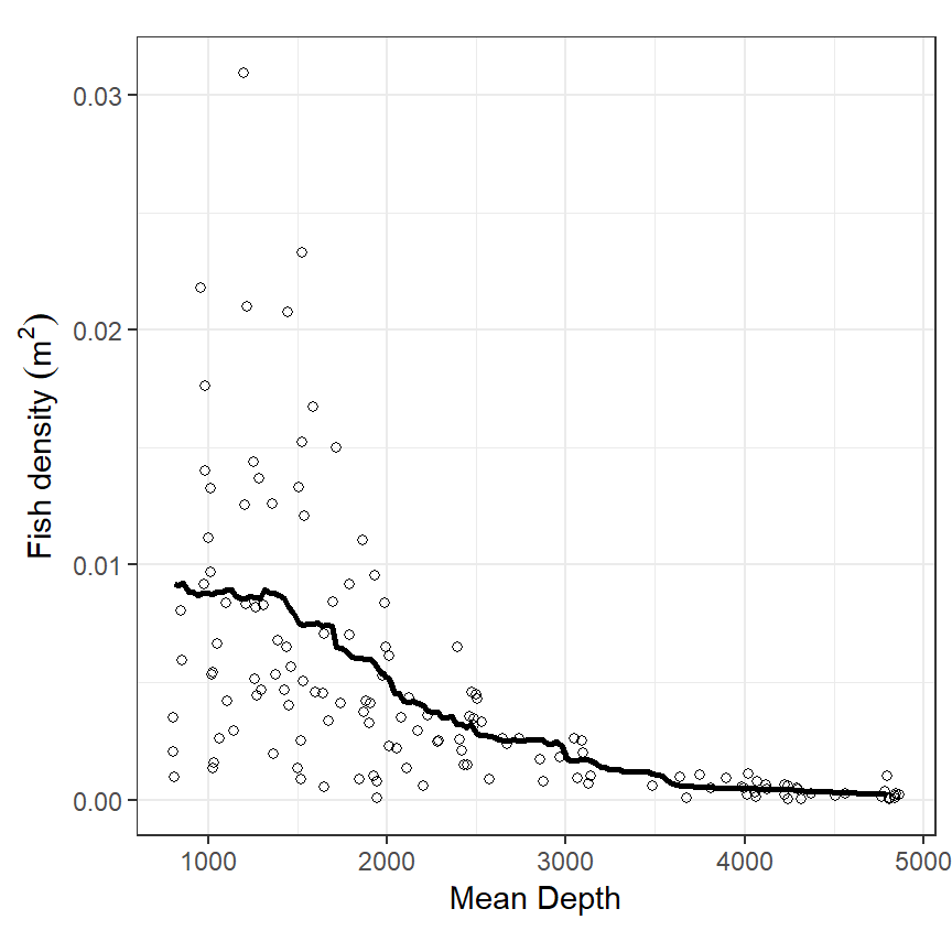
図2.10: Estimated moving average smoother
2.2.4.2 局所回帰(LOESS)
移動平均ではギザギラのラインが推定されるが、LOESSではよりスムーズなラインを引くことができる。局所回帰は推定値を求めたいポイントの前後にある特定の範囲(あるいは個数?)のデータだけを用いて多項式回帰を行い(多くのソフトでデフォルトでは2次の項までを含む)、その予測値を推定値とする方法である。移動平均と同様に一定間隔のポイントに対してこれを行うことで、平滑化した曲線を描く。
Rでは、loess関数で推定を行うことができる。span =で各ポイントでの推定に用いるデータの割合を指定できる(デフォルトは0.75)。図2.11はspanを0.1, 0.5, 1にした場合に描けるモデルから推定された平滑化曲線である。1のときは、全データを使用した多項式回帰と同じ結果である。移動平均でもLOESSでも、推定を行う際に使用するデータの範囲を変えると結果も大きく変わるので注意が必要である。
M2_3_a <- loess(Dens ~ MeanDepth, data = fish, span = 0.1)
M2_3_b <- loess(Dens ~ MeanDepth, data = fish, span = 0.5)
M2_3_c <- loess(Dens ~ MeanDepth, data = fish, span = 1)

pred_M2_3_a <- predict(M2_3_a, se = TRUE,
                       newdata = data.frame(MeanDepth = seq(800, 4865, length.out = 100))) %>%
  data.frame() %>%
  bind_cols(data.frame(MeanDepth = seq(800, 4865, length.out = 100))) %>%
  mutate(upper = fit + qt(0.975, df = df)*se.fit,
         lower = fit - qt(0.975, df = df)*se.fit,
         span = 0.1)

pred_M2_3_b <- predict(M2_3_b, se = TRUE,
                       newdata = data.frame(MeanDepth = seq(800, 4865, length.out = 100))) %>%
  data.frame() %>%
  bind_cols(data.frame(MeanDepth = seq(800, 4865, length.out = 100))) %>%
  mutate(upper = fit + qt(0.975, df = df)*se.fit,
         lower = fit - qt(0.975, df = df)*se.fit,
         span = 0.5)

pred_M2_3_c <- predict(M2_3_c, se = TRUE,
                       newdata = data.frame(MeanDepth = seq(800, 4865, length.out = 100))) %>%
  data.frame() %>%
  bind_cols(data.frame(MeanDepth = seq(800, 4865, length.out = 100))) %>%
  mutate(upper = fit + qt(0.975, df = df)*se.fit,
         lower = fit - qt(0.975, df = df)*se.fit,
         span = 1)

bind_rows(pred_M2_3_a, pred_M2_3_b, pred_M2_3_c) %>%
  mutate(span = str_c("span = ", span)) %>%
  ggplot(aes(x = MeanDepth, y = fit))+
  geom_line()+
  geom_ribbon(aes(ymin = lower, ymax = upper),
              alpha = 0.3)+
  geom_point(data = fish,
             aes(y = Dens),
             shape = 1)+
  facet_rep_wrap(~ span)+
  theme_bw(base_size = 12)+
  theme(aspect.ratio = 1)+
  labs(x = "Mean Depth", y = expression(paste("Fish density"," ", (m^2))))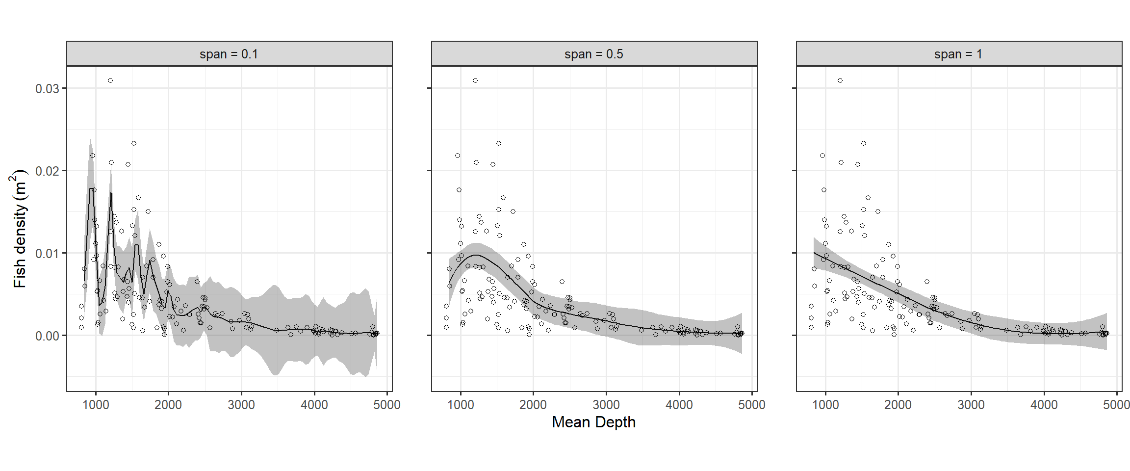
図2.11: LOESS smoother using a span of 0.1, 0.5, and 1.
2.2.5 Packages for smoothing
Rには、平滑化を行うことができるパッケージが複数存在する。例えば、gamパッケージ(Hastie and Hastie 2018)、mgcvパッケージ(Wood and EPSRC 2007)、gamlssパッケージ(Rigby et al. 2019)などがある。それぞれのパッケージに長所と短所があり、gamはLOESSを用いる際に使いやすく、mgvcはより発展的な手法に対して使いやすい。gamlssはより広い分布に対して用いることができる。本稿では主にmgcvパッケージを用いる。
mgvcパッケージでは様々な手法を用いた平滑化を行うことができるが、自身のデータに対してどの方法を用いるかを決めるためにはこうした手法について知っていなければならない。こうした手法については、第(3)章で詳しく学ぶ。
2.3 Allpying GAM in R using the mgcv package
本節では、mgvcパッケージを用いてGAMを適用する方法を学ぶ。まず、gam関数を用いて式(2.1)を以下のように適用する。なお、fx = TRUE、k = 5というのは有効自由度4の平滑化関数が用いられていることを示しているが、詳しくは次章で説明する。
gam関数はthin plate regression splineといわれる方法を用いている。有効自由度は曲線の形を決める値であり(calibration value)、1だと直線になり大きくなるほどより非線形な形になる。自由度4は古典的なパッケージでデフォルトとしてよく使われている値であり、推定された曲線は3次の項までを含む多項式回帰によるものと似ている。次節(2.4)ではcross validationを用いてどの自由度が最も適切か決める方法を学ぶ。
summary関数でモデルの結果の概要を得ることができる。
##
## Family: gaussian
## Link function: identity
##
## Formula:
## Dens ~ s(MeanDepth, fx = TRUE, k = 5)
##
## Parametric coefficients:
##              Estimate Std. Error t value Pr(>|t|)
## (Intercept) 0.0047137  0.0003616   13.04   <2e-16 ***
## ---
## Signif. codes:  0 '***' 0.001 '**' 0.01 '*' 0.05 '.' 0.1 ' ' 1
##
## Approximate significance of smooth terms:
##              edf Ref.df     F  p-value
## s(MeanDepth)   4      4 22.12 3.27e-14 ***
## ---
## Signif. codes:  0 '***' 0.001 '**' 0.01 '*' 0.05 '.' 0.1 ' ' 1
##
## R-sq.(adj) =  0.367   Deviance explained = 38.4%
## GCV = 1.9894e-05  Scale est. = 1.9218e-05  n = 147
切片の推定値は0.0047なので、モデル式は以下のように書ける。
\[
Dens_i = 0.0047 + f(Depth_i)
\]
また、結果からはモデルが分散の36.9%を説明すること、推定された残差が従う正規分布の分散が\(1.908 \times 10^{-5}\)であることも分かる。
smoother(\(f(Dens_i)\))の有意性(Approximate significance of smooth term)は、以下のF値によって計算されている。なお、\(RSS_1、RSS_2\)はそれぞれsmootherがないモデルとあるモデルの残差平方和、\(pとq\)はそれぞれsmootherがあるモデルとないモデルの自由度、\(N\)はサンプル数である。もしモデルが前提を満たすならば、Fは自由度\(N-p\)と\(p-q\)のF分布に従う。
\[ F = \frac{(RSS_1 - RSS_2)/(p-q)}{RSS_2/(N-p)} \]
モデルによって推定された曲線は以下のようになる(図2.12)。mgvcパッケージで推定した結果は、gratiaパッケージを用いると簡単に描画することができる。
dataM2_4 <- data.frame(MeanDepth = seq(800, 4865, length.out = 100))

## 予測値を算出
pred_M2_4_4 <- fitted_values(M2_4, data = dataM2_4) %>%
  mutate(df = 4)

## 描画
pred_M2_4_4 %>%
  ggplot(aes(x = MeanDepth, y = fitted))+
  geom_line()+
  geom_ribbon(aes(ymin = lower, ymax = upper),
              alpha = 0.3) +
  geom_point(data = fish,
             aes(y = Dens),
             shape = 1)+
  coord_cartesian(ylim = c(0,0.032))+
  theme_bw(base_size = 12)+
  theme(aspect.ratio = 1)+
  labs(x = "Mean Depth", y = expression(paste("Fish density"," ", (m^2))))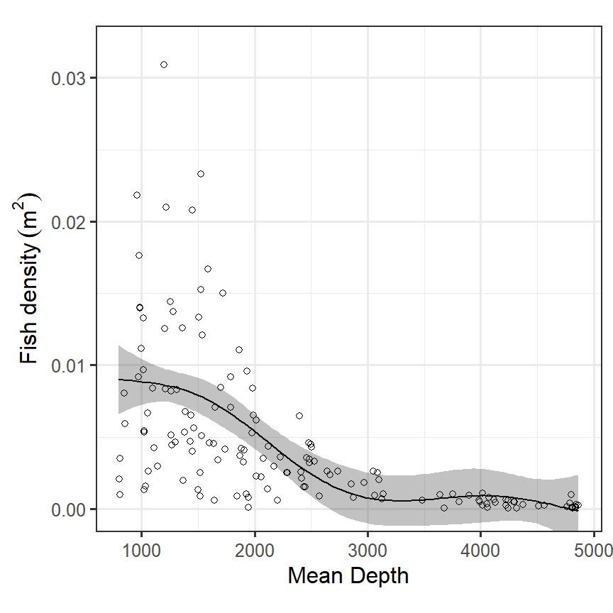
図2.12: Fitted values obtained by the GAM.
2.4 Cross validation
前節では自由度4で分析を行ったが、自由度はほかの値に設定することも可能である。図2.13は様々な自由度を用いたモデルの推定結果を図示したものである。どのようにして最適な自由度を選べばよいだろうか?
## df = 2
M2_4_2 <- gam(Dens ~ s(MeanDepth, fx = TRUE, k = 3),
            data = fish)

pred_M2_4_2 <- fitted_values(M2_4_2, data = dataM2_4) %>%
  mutate(df = 2)

## df = 3
M2_4_3 <- gam(Dens ~ s(MeanDepth, fx = TRUE, k = 4),
            data = fish)

pred_M2_4_3 <- fitted_values(M2_4_3, data = dataM2_4) %>%
  mutate(df = 3)

## df = 5
M2_4_5 <- gam(Dens ~ s(MeanDepth, fx = TRUE, k = 6),
            data = fish)

pred_M2_4_5 <- fitted_values(M2_4_5, data = dataM2_4) %>%
  mutate(df = 5)

## df = 7
M2_4_7 <- gam(Dens ~ s(MeanDepth, fx = TRUE, k = 8),
            data = fish)

pred_M2_4_7 <- fitted_values(M2_4_7, data = dataM2_4) %>%
  mutate(df = 7)

## df = 9
M2_4_9 <- gam(Dens ~ s(MeanDepth, fx = TRUE, k = 10),
            data = fish)

pred_M2_4_9 <- fitted_values(M2_4_9, data = dataM2_4) %>%
  mutate(df = 9)

## 描画
bind_rows(pred_M2_4_2, pred_M2_4_3, pred_M2_4_4, pred_M2_4_5, pred_M2_4_7,pred_M2_4_9) %>%
  mutate(df = str_c("df = ",df)) %>%
  ggplot(aes(x = MeanDepth, y = fitted))+
  geom_line()+
  geom_ribbon(aes(ymin = lower, ymax = upper),
              alpha = 0.3) +
  geom_point(data = fish,
             aes(y = Dens),
             shape = 1)+
  coord_cartesian(ylim = c(0,0.032))+
  theme_bw(base_size = 12)+
  theme(aspect.ratio = 1)+
  labs(x = "Mean Depth", y = expression(paste("Fish density"," ", (m^2)))) +
  facet_rep_wrap(~df, repeat.tick.labels = TRUE)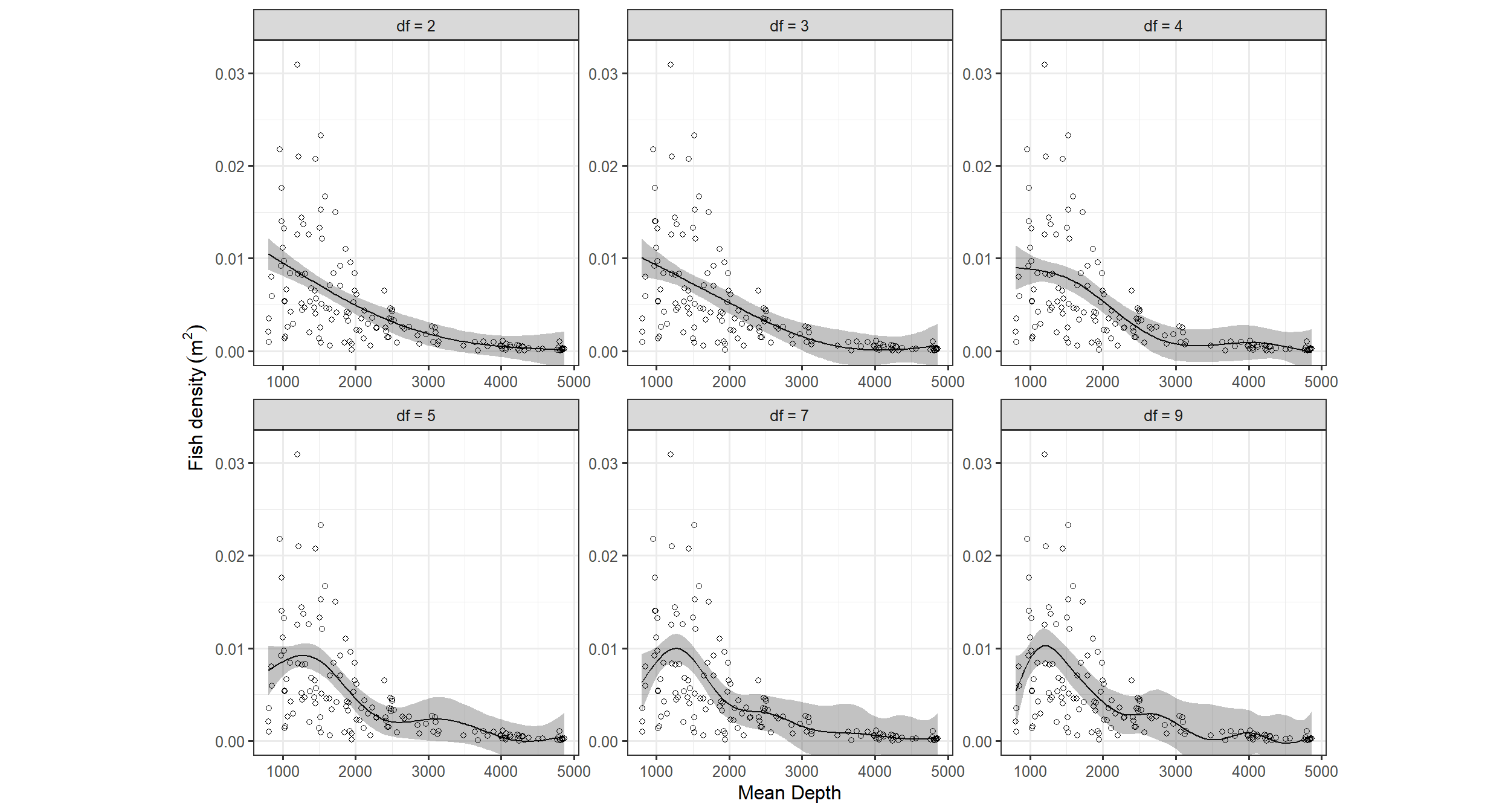
図2.13: Fitted values obtained by the GAM using 2, 3, 4, 5, 7, 9 degrees of freedom.
gam関数では、fx =とk =を書かなければ自動的に交差検証(cross validation)を実行し、最適な自由度を探してくれる。下記のように、最適な自由度は5.62ということになる。
##
## Family: gaussian
## Link function: identity
##
## Formula:
## Dens ~ s(MeanDepth)
##
## Parametric coefficients:
##              Estimate Std. Error t value Pr(>|t|)
## (Intercept) 0.0047137  0.0003561   13.24   <2e-16 ***
## ---
## Signif. codes:  0 '***' 0.001 '**' 0.01 '*' 0.05 '.' 0.1 ' ' 1
##
## Approximate significance of smooth terms:
##                edf Ref.df    F p-value
## s(MeanDepth) 5.621  6.723 14.1  <2e-16 ***
## ---
## Signif. codes:  0 '***' 0.001 '**' 0.01 '*' 0.05 '.' 0.1 ' ' 1
##
## R-sq.(adj) =  0.386   Deviance explained = 40.9%
## GCV = 1.9514e-05 Scale est. = 1.8635e-05 n = 147推定結果をもとに描いた平滑化曲線は以下のようになる(図2.14)。
pred_M2_5 <- smooth_estimates(M2_5, data = dataM2_4) %>%
  ## 95%信頼区間を算出
  add_confint() %>%
  mutate(est = est + coef(M2_5)[[1]],
         lower_ci = lower_ci + coef(M2_5)[[1]],
         upper_ci = upper_ci + coef(M2_5)[[1]]) %>%
  mutate(df = 4)

## 描画
pred_M2_5 %>%
  ggplot(aes(x = MeanDepth, y = est))+
  geom_line()+
  geom_ribbon(aes(ymin = lower_ci, ymax = upper_ci),
              alpha = 0.3) +
  geom_point(data = fish,
             aes(y = Dens),
             shape = 1)+
  coord_cartesian(ylim = c(-0.001,0.032))+
  theme_bw(base_size = 12)+
  theme(aspect.ratio = 1)+
  labs(x = "Mean Depth", y = expression(paste("Fish density"," ", (m^2))))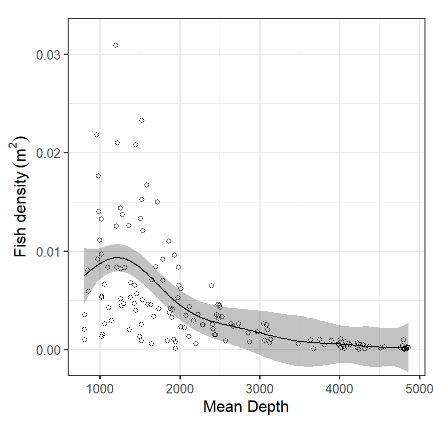
図2.14: Fitted values obtained by the GAM.
それでは、交差検証とは何だろうか?smoother\(f(Depth_i)\)の推定値を\(\hat{f}(Depth_i)\)とするとき、推定値が真のsmootherとどれほど近いかは以下の式で表せる。
\[ M = \frac{1}{n}\sum_{i = 1} ^n (f(Depth_i) - \hat{f}(Depth_i))^2 \]
もし私たちが真の\(f(Depth_i)\)を知っているならば、Mが最小になるように\(\hat{f}(Depth_i)\)を推定することができるが、真のsmootherを知ることはできない。そのため、私たちは\(M\)を何か計算可能なもので代用する必要がある。
方法としては、交差検証、一般化交差検証(generalized cross validation)、頑強なリスク推定(unbiased risk estimator)、Marrow’s Cpなどがある。gam関数では、通常の加法モデルを適用するか、一般化加法モデルを適用するかによってこれらのいずれかが用いられる。本節では、通常の交差検証(ordinary cross validation: OCV)について簡単な解説を行う。
交差検証のスコア\(V_0\)は以下の式で与えられる。\(f^{-i}(Depth_i)\)は\(i\)番目のデータ以外のデータから推定されたsmootherの推定値を表す。\(V_0\)を最小にするようにsmootherの推定値を求める。
\[ V_0 = \frac{1}{n}\sum_{i = 1} ^n (Depth_i -f^{-i}(Depth_i))^2 \]
理論的に、\(V_0\)の期待値は\(M\)の期待値に分散\(\sigma^2\)を足した値に近似できる。
\[ E[V_0] \approx E[M] + \sigma^2 \]
これを計算するのは負荷が大きいため、通常はgeneralized cross validation scoreというものを用いることでshortcutを行う。詳細については第3章で解説を行う。データ数が50未満の場合は多重共線性やデータの非独立性によって交差検証の結果に問題が生じることがある。そのため、交差検証の結果をきちんと確認することが必要である。
2.5 Model validation
2.5.1 Normality and homogeneity
GAMでは重回帰分析のときと同様に残差を抽出し、その正規性や等分散性、独立性、影響のある観察の有無を確認しなければならない。
gratiaパッケージでは、appraise関数でQQプロット、残差 vs 予測値、残差のヒストグラム、実測値 vs 予測値のプロットを作成してくれる(図2.15)。なお、それぞれのグラフはqq_plot()、residuals_linpred_plot()、residuals_hist_plot()、observed_fitted_plotで個別に作成できる。
この結果から、等分散性や残差の正規性が成立していないことが分かる。
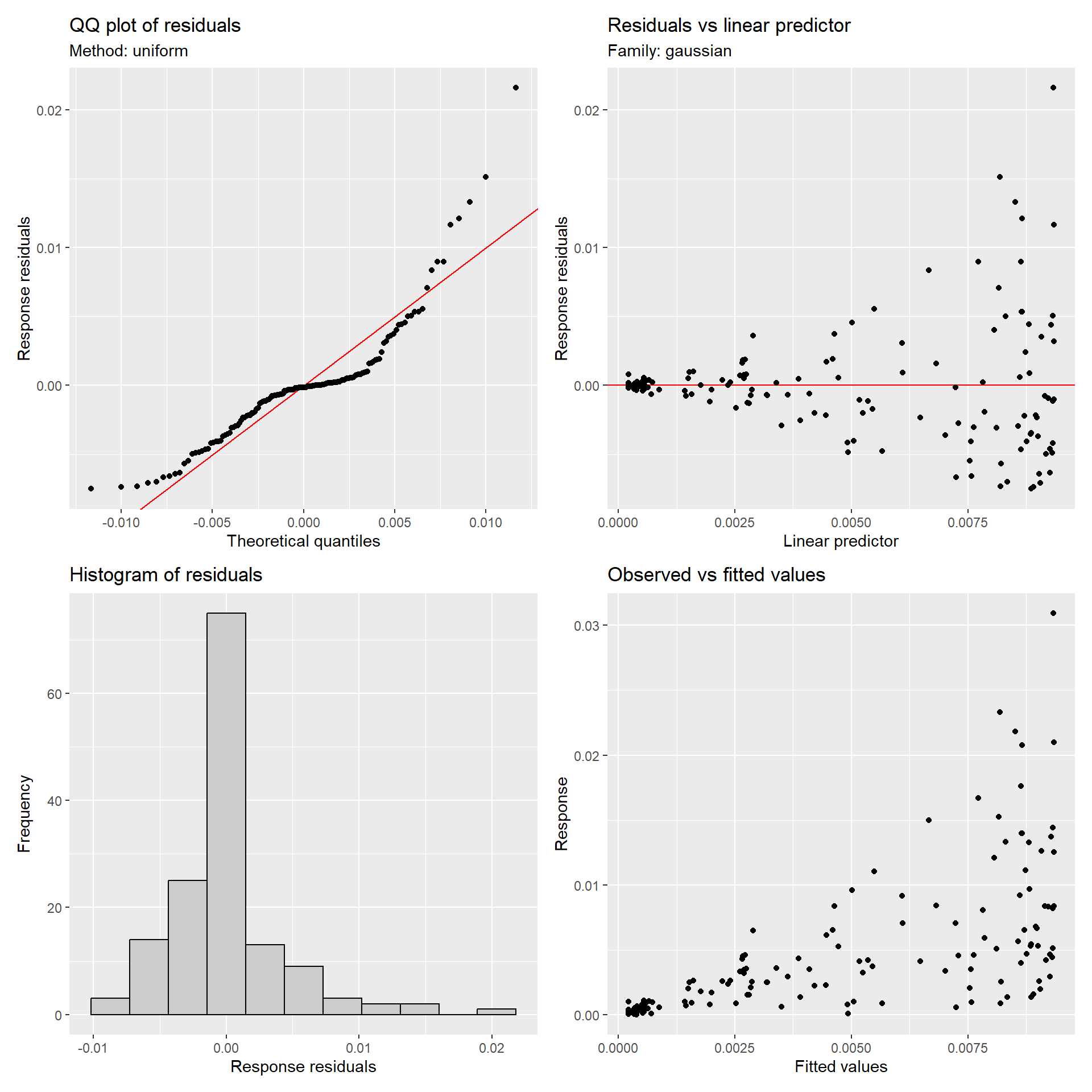
図2.15: Model diagnosis using gratia package.
手動で残差 vs 予測値、残差のヒストグラムは以下のように作成できる(図2.16)。
data.frame(res <- resid(M2_5),
           fitted = fitted(M2_5)) -> diag_M2_5

diag_M2_5 %>%
  ggplot(aes(x = fitted,y = res))+
  geom_point()+
  geom_hline(yintercept = 0, color = "red")+
  theme_bw()+
  theme(aspect.ratio = 1)+
  labs(x = "Fitted value", y = "Residuals") -> p_diag_M2_5_a

diag_M2_5 %>%
  ggplot(aes(x = res))+
  geom_histogram(fill = "white", color = "black")+
  theme_bw()+
  theme(aspect.ratio = 1)+
  labs(x = "Residuals", y = "Frequancy") -> p_diag_M2_5_b

p_diag_M2_5_a + p_diag_M2_5_b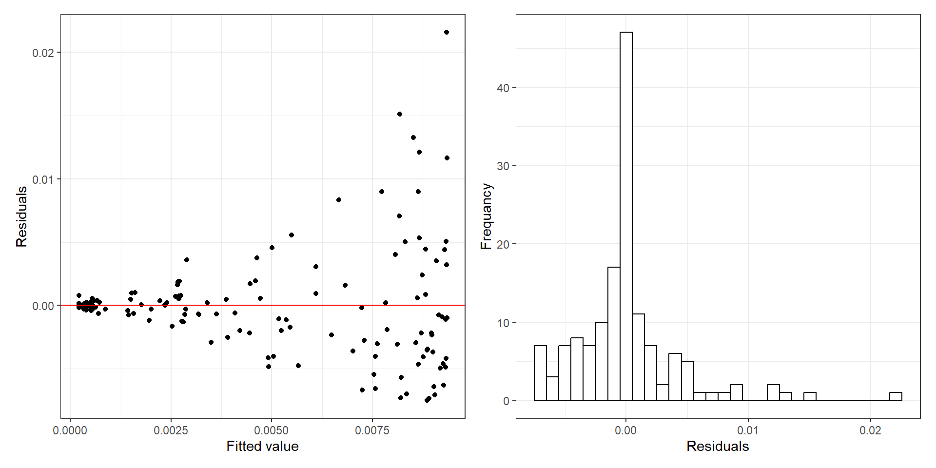
図2.16: Model diagnosis of GAM.
2.5.2 Independence
残差の独立性を確認するため、残差と説明変数などの変数の関連をプロットする(図2.17)。水深との関連については(A)、等分散性の仮定が満たされていないことを除けば、特にパターンは見られない。もし水深との関連にもパターンがみられていたら、GAMの自由度を上げることでこの問題を解決できる。
一方で、期間との関連についてはパターンがみられ、期間2の残差がほとんど0を下回っている。このことは、Periodをモデルに加えた方がいいことを示唆している。
data.frame(res = resid(M2_5),
           MeanDepth = fish$MeanDepth) %>%
  ggplot(aes(x = MeanDepth, y = res))+
  geom_point(shape = 1)+
  theme_bw()+
  theme(aspect.ratio = 1)+
  labs(x = "Depth", y = "Residuals", title = "A") -> p_ind_M2_5_a

data.frame(res = resid(M2_5),
           Period = as.factor(fish$Period)) %>%
  ggplot(aes(x = Period, y = res))+
  geom_boxplot()+
  theme_bw()+
  theme(aspect.ratio = 1)+
  labs(x = "Period", y = "Residuals", title = "B") -> p_ind_M2_5_b

p_ind_M2_5_a + p_ind_M2_5_b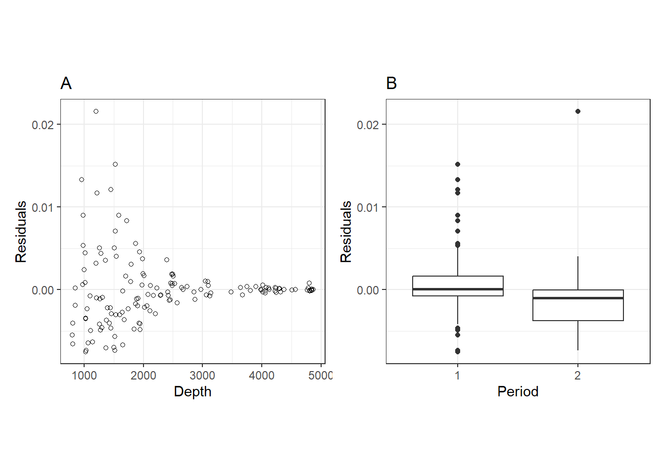
図2.17: A: residuals versus depth. B: residuals versus period
残差に空間的な相関があるかを調べるため、各データポイントで調査が行われた場所と残差の大きさの関連を示したものが図2.18である。残差の大きさが点の色と大きさで表されている。このデータだけではいまいち解釈がしにくい。
data.frame(res = resid(M2_5),
           x = fish$Xkm,
           y = fish$Ykm) %>%
  ggplot(aes(x = x, y = y))+
  geom_point(aes(color = res, size = res),
             alpha = 0.5)+
  scale_size(range = c(1,7))+
  theme_bw()+
  theme(aspect.ratio = 1)+
  labs(x = "X-coordinates", y = "Y-coordinates")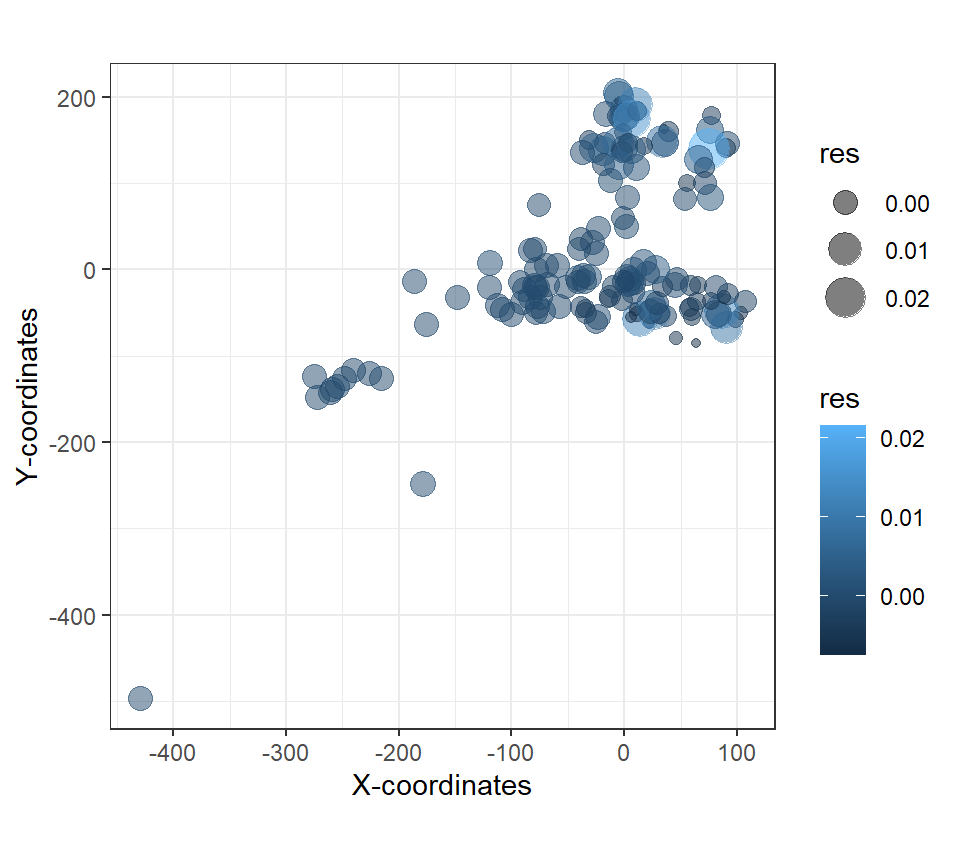
図2.18: Bubble plot of the residuals.
このようなときに使えるのがバリオグラム(variogram)である。バリオグラムは以下の手順で作成する。なお、通常dは離散的に選択する。
- 全てのサイト間の距離を計算する。
- 距離がある特定の値dであるサイトの全組み合わせについて残差の差の二乗を計算し、それの平均値を算出する。
- これを全ての距離について行い、距離と平均値の関係をプロットする。
もし残差が空間的に独立なのであれば、算出された平均値は水平に分布する。
Rではgstatパッケージで以下のように算出できる。図で表したものが図2.19である。図からは150m以上離れるとsemi-variogram値(縦軸)が大きくなる傾向があることが分かる。このパターンは、他の変数や交互作用をモデルに含めることで解消できるかもしれない。
fish_cor <- fish
## coordinateを作成
sp::coordinates(fish_cor) <- ~ Xkm + Ykm

## 算出
vario_M2_5 <- gstat::variogram(resid(M2_5) ~ 1, fish_cor)

## 作図
vario_M2_5 %>%
  ggplot(aes(x = dist, y = gamma))+
  geom_point(size = 3)+
  theme_bw()+
  theme(aspect.ratio = 1)+
  labs(x = "Distance (km)", y = "semivariogram")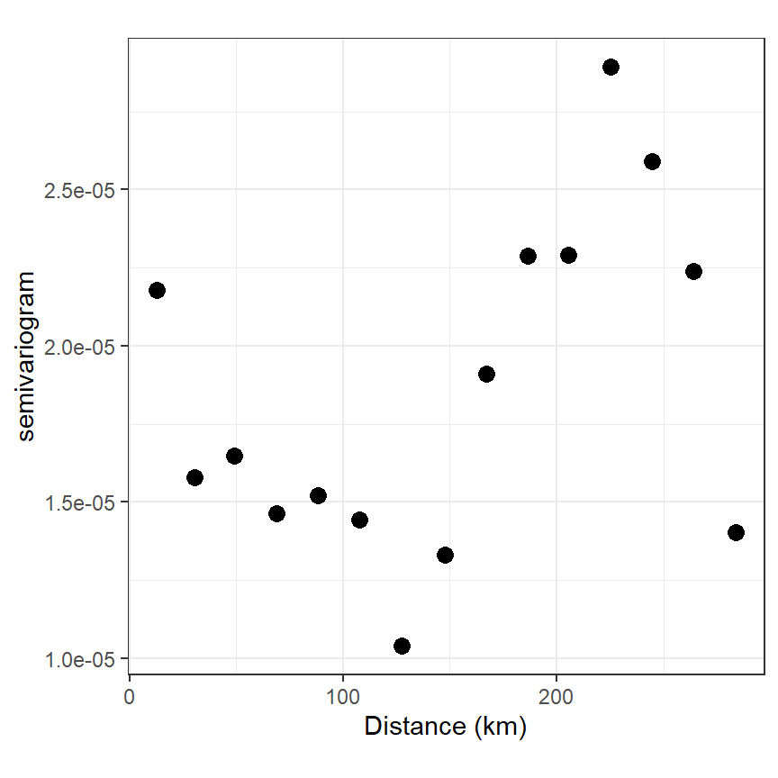
図2.19: Semi-variogram of the residuals of the GAM.
この分析の問題点は深さが考慮されていない点である。2地点間のxy平面上の距離が近くても、深さが違えば実際の距離は最大で5km近く離れている可能性がある。
2.5.3 Influential observations
GAMではcook’s distanceは算出できないが、各観測値の影響力の強さは全データを用いたモデルから推定されたsmoother(\(\hat{f}(Depth_i)\))からその観測値以外のデータを用いたモデルから推定されたsmoother(\(f^{-i}(Depth_i)\))を引いた値の二乗の合計値を算出することで求めることができる。各観測値について影響力の大きさは以下のように定式化できる。
\[ I_i = \sum_{i = 1}^n (\hat{f}(Depth_i) - f^{-i}(Depth_i))^2 \]
Rでは以下のように計算できる。
nd <- data.frame(MeanDepth = seq(min(fish$MeanDepth), max(fish$MeanDepth), length.out = 150))
pred_M2_5 <- predict(M2_5, newdata = nd, type = "terms")

I <- vector()

for(i in 1:nrow(fish)){
  M2_5.i <- gam(Dens ~ s(MeanDepth), data = fish %>% filter(Site != fish[i,1][[1]]))
  pred_M2_5.i <- predict(M2_5.i, newdata = nd, type = "terms")
  I[i] <- sum((pred_M2_5[1:150] - pred_M2_5.i[1:150])^2)
}各ポイントの影響力の大きさをサイズにしてプロットしたのが図2.20である。いくつか影響力の高そうな点があるが、それが有意に大きいのか否かを言うことはできない。
fish %>%
  mutate(I = I) %>%
  ggplot(aes(x = MeanDepth, y = Dens))+
  geom_point(aes(size = I))+
  theme_bw()+
  theme(aspect.ratio = 1,
        legend.position = "none")+
  labs(x = "Depth", y = expression(paste("Fish density"," ", (m^2))))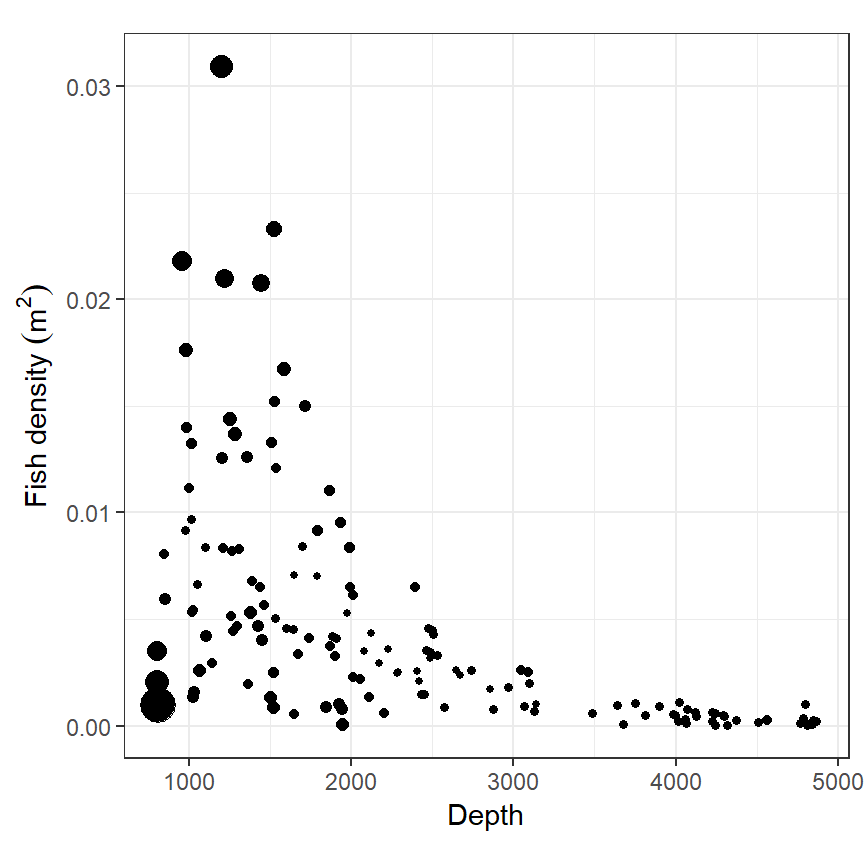
図2.20: Scatterplot of fish density versus depth. The size of an observation point is proportional to its influence on the shape of the smoother.
2.6 Extending the GAM with more covariates
2.6.1 GAM with smoother and a normal covariate
GAMでも通常の線形モデルと同様に2つ以上の説明変数や交互作用を含めることができる。ここでは、これまでのモデルでは考慮できなかった調査期間(Period)と調査期間と水深(MeanDepth)の交互作用を入れることで、調査期間ごとに水深と魚の密度の関係が変わっているのかを調べるモデルを作成する。本節では交互作用なしとありのモデルを作成し、どちらがより良いモデルかを検討する。
交互作用なしモデルのモデル式は以下のようになる。このモデルでは、水深と魚の密度の関連はいずれの期間でも同じだが、その平均が期間によって異なることを仮定している。
\[
\begin{aligned}
Dnes_i &= \alpha + f(Depth_i) + \beta \times Period_i + \epsilon_i \\
\epsilon_i &\sim N(0,\sigma^2)
\end{aligned}
\]
モデルはRで以下のように実行できる。
fish <- fish %>% mutate(Period = as.factor(Period))
M2_6 <- gam(Dens ~ s(MeanDepth) + Period, data = fish)
結果は以下の通り。
##
## Family: gaussian
## Link function: identity
##
## Formula:
## Dens ~ s(MeanDepth) + Period
##
## Parametric coefficients:
##               Estimate Std. Error t value Pr(>|t|)
## (Intercept)  0.0054572  0.0004291  12.716  < 2e-16 ***
## Period2     -0.0021859  0.0007433  -2.941  0.00383 **
## ---
## Signif. codes:  0 '***' 0.001 '**' 0.01 '*' 0.05 '.' 0.1 ' ' 1
##
## Approximate significance of smooth terms:
##                edf Ref.df     F p-value
## s(MeanDepth) 5.566  6.664 14.85  <2e-16 ***
## ---
## Signif. codes:  0 '***' 0.001 '**' 0.01 '*' 0.05 '.' 0.1 ' ' 1
##
## R-sq.(adj) =  0.417   Deviance explained = 44.4%
## GCV = 1.8637e-05  Scale est. = 1.7677e-05  n = 147
モデルの推定結果からそれぞれの期間について以下のような式が書ける。
\[
\begin{aligned}
Period1: Dens_i &= 0.0054 + f(Depth_i) \\
Period2: Dens_i &= 0.0032 + f(Depth_i)
\end{aligned}
\]
モデルの結果を図示したのが図2.21である。
nd <- crossing(MeanDepth = seq(800, 4650, length.out = 100),
               Period = as.factor(c(1,2)))

fitted_values(M2_6, data = nd, scale = "response") %>%
  ggplot(aes(x = MeanDepth))+
  geom_point(data = fish,
             aes(y = Dens, fill = Period),
             shape = 21)+
  geom_line(aes(y = fitted, linetype = Period),
            linewidth = 1)+
  scale_fill_manual(values = c("white","black"))+
  scale_linetype_manual(values = c("solid","dashed"))+
  theme_bw()+
  theme(aspect.ratio = 1)+
  labs(x = "Depth", y = expression(paste("Fish density"," ", (m^2))))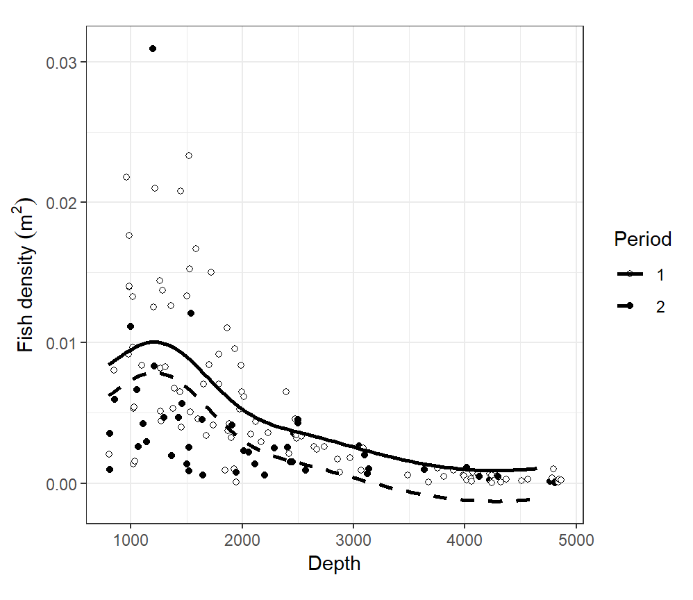
図2.21: Visualisation of the GAM that contains a smoother of depth and period as a factor.
2.6.2 GAM with interaction terms; first implement
GAMで交互作用を含める場合、モデルは以下のようになる。\(f_1(Depth_i)\)と\(f_2(Depth_i)\)はそれぞれの期間ごとのsmootherを表す。
\[ \begin{aligned} Dnes_i &= \alpha + f_1(Depth_i) +f_2(Depth_i) + \beta \times Period_i + \epsilon_i \\ \epsilon_i &\sin N(0,\sigma^2) \end{aligned} \]
このモデルはRでは以下のように実行できる。
推定結果は以下の通り。期間ごとにsmootherを推定しているので、それぞれのsmootherの自由度が異なる。期間2は自由度が1.078なのでほとんど直線に近いことになる。
##
## Family: gaussian
## Link function: identity
##
## Formula:
## Dens ~ s(MeanDepth, by = Period) + Period
##
## Parametric coefficients:
##               Estimate Std. Error t value Pr(>|t|)
## (Intercept)  0.0054405  0.0004286  12.693  < 2e-16 ***
## Period2     -0.0022054  0.0007324  -3.011  0.00309 **
## ---
## Signif. codes:  0 '***' 0.001 '**' 0.01 '*' 0.05 '.' 0.1 ' ' 1
##
## Approximate significance of smooth terms:
##                        edf Ref.df     F  p-value
## s(MeanDepth):Period1 4.169  5.094 17.18  < 2e-16 ***
## s(MeanDepth):Period2 1.078  1.151 10.33 0.000913 ***
## ---
## Signif. codes:  0 '***' 0.001 '**' 0.01 '*' 0.05 '.' 0.1 ' ' 1
##
## R-sq.(adj) =  0.419   Deviance explained = 44.4%
## GCV = 1.8547e-05  Scale est. = 1.7632e-05  n = 147
推定結果から、各期間の魚の密度と水深の関係は以下のようになる。
\[
\begin{aligned}
Period1: Dens_i &= 0.0054 + f_1(Depth_i) \\
Period2: Dens_i &= 0.0032 + f_2(Depth_i)
\end{aligned}
\]
推定結果を図示したのが図2.22である。
fitted_values(M2_7, data = nd, scale = "response") %>%
  mutate(Period = str_c("Period ", Period)) %>%
  ggplot(aes(x = MeanDepth))+
  geom_point(data = fish %>% mutate(Period = str_c("Period ", Period)),
             aes(y = Dens, fill = Period),
             shape = 21)+
    geom_line(aes(y = fitted, linetype = Period),
            linewidth = 1)+
  scale_fill_manual(values = c("white","black"))+
  scale_linetype_manual(values = c("solid","dashed"))+
  theme_bw()+
  theme(aspect.ratio = 1,
        legend.position = "none")+
  labs(x = "Depth", y = expression(paste("Fish density"," ", (m^2))))+
  facet_wrap(~Period)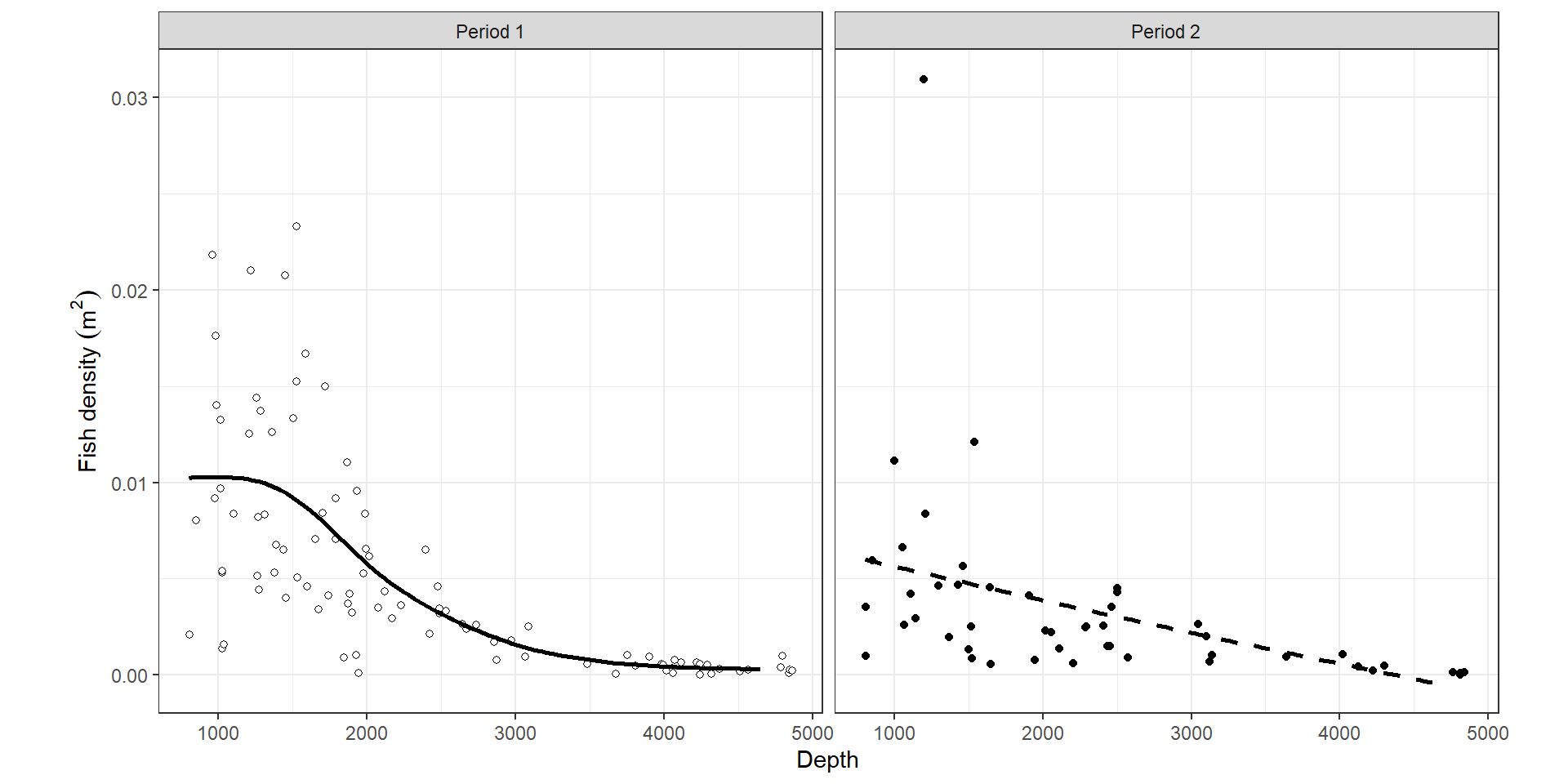
図2.22: Visualisation of the GAM that contains a smoother of depth and period as a factor.
2.6.3 GAM with interaction; third implementation
期間ごとに異なるsmootherを推定するもう一つの方法として、以下のモデルを使うこともできる。ここで、\(f(Depth)\)は両期間に共通するsmoother、、\(f_2(Depth)\)は期間2のみに適用されるsmootherである。
\[ \begin{aligned} Dens_i &= \alpha + f(Depth_i) +f_2(Depth_i) + \epsilon_i \\ \epsilon_i &\sim N(0,\sigma^2) \end{aligned} \]
このモデルはRで以下のように実行できる。モデル式の中にモデルM2_7のように\(Period\)が単独で説明変数として入っていない点には注意が必要である。これは、gamでs(MeanDepth, by = as.numeric(Period == "2"))のように指定を行う場合はsmootherが0で中心化されていないからである(それ以外の場合は0で中心化されている)。
モデルの結果は以下のとおりである。期間2だけのsmootherも有意であるので、期間1と2でsmootherが有意に異なることが分かる。モデルM2_7と異なるのは、このように水深と魚の密度の関連が期間ごとに有意に異なるのかを検定できる点である。
##
## Family: gaussian
## Link function: identity
##
## Formula:
## Dens ~ s(MeanDepth) + s(MeanDepth, by = as.numeric(Period ==
##     "2"))
##
## Parametric coefficients:
##              Estimate Std. Error t value Pr(>|t|)
## (Intercept) 0.0054462  0.0004248   12.82   <2e-16 ***
## ---
## Signif. codes:  0 '***' 0.001 '**' 0.01 '*' 0.05 '.' 0.1 ' ' 1
##
## Approximate significance of smooth terms:
##                                          edf Ref.df      F p-value
## s(MeanDepth)                           4.714  5.729 15.697 < 2e-16 ***
## s(MeanDepth):as.numeric(Period == "2") 2.000  2.000  6.737 0.00161 **
## ---
## Signif. codes:  0 '***' 0.001 '**' 0.01 '*' 0.05 '.' 0.1 ' ' 1
##
## R-sq.(adj) =  0.428   Deviance explained = 45.4%
## GCV = 1.8319e-05  Scale est. = 1.7358e-05  n = 147
推定結果から、各期間の魚の密度と水深の関係は以下のようになる。
\[
\begin{aligned}
Period1: Dens_i &= 0.0054 + f(Depth_i) \\
Period2: Dens_i &= 0.0054 + f(Depth_i) + f_2(Depth_i)
\end{aligned}
\]
推定結果を図示したのが図2.23である。
fitted_values(M2_8, data = nd, scale = "response") %>%
  mutate(Period = str_c("Period ", Period)) %>%
  ggplot(aes(x = MeanDepth))+
  geom_point(data = fish %>% mutate(Period = str_c("Period ", Period)),
             aes(y = Dens, fill = Period),
             shape = 21)+
    geom_line(aes(y = fitted, linetype = Period),
            linewidth = 1)+
  scale_fill_manual(values = c("white","black"))+
  scale_linetype_manual(values = c("solid","dashed"))+
  theme_bw()+
  theme(aspect.ratio = 1,
        legend.position = "none")+
  labs(x = "Depth", y = expression(paste("Fish density"," ", (m^2))))+
  facet_wrap(~Period)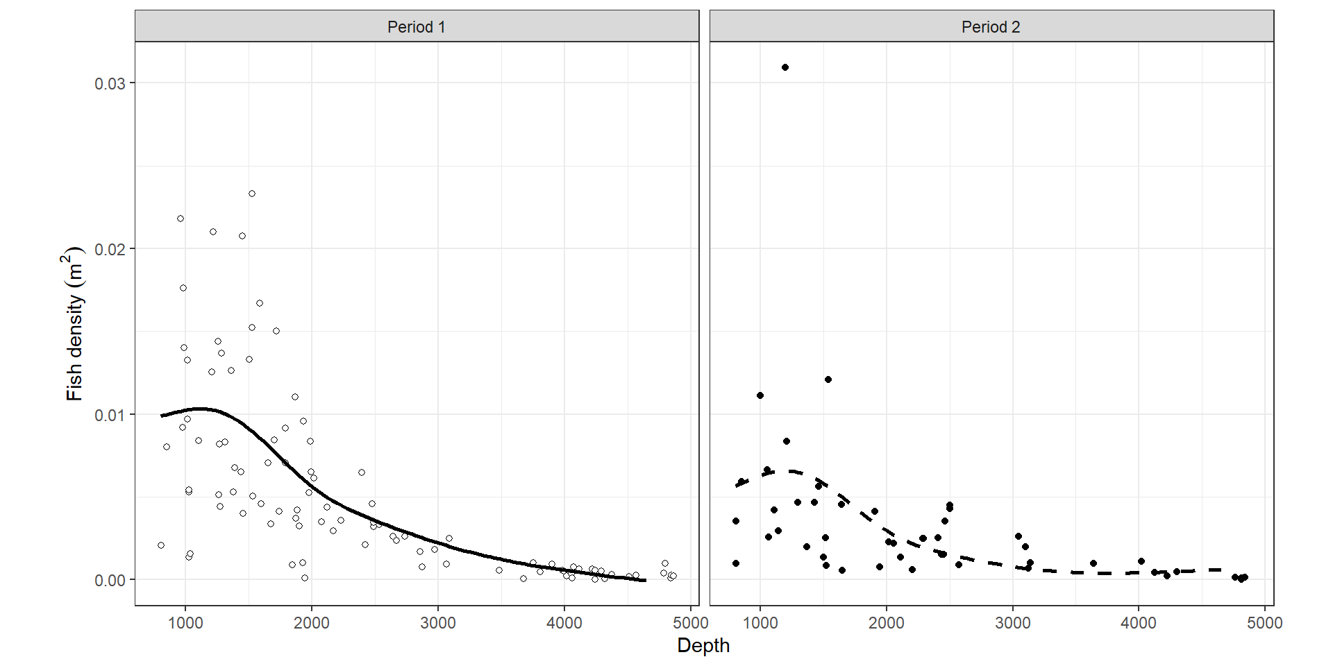
図2.23: Visualisation of the GAM that contains a smoother of depth and period as a factor.
これまでに適用した交互作用を含むモデル(M2_7とM2_8)のモデル診断を行うと、いずれも等分散性や正規性の仮定を満たしていないことが分かる(図2.24と図(fig:fig-gam-diagnosis-M2-8))。
このようなとき、取りうる手段は(1) 変数を変換する、(2)等分散性を許容できる推定方法(GLSなど)を用いる、(3) (1)と(2)を組み合わせた方法を用いる、などがある。以下では、こうした方法について議論する。
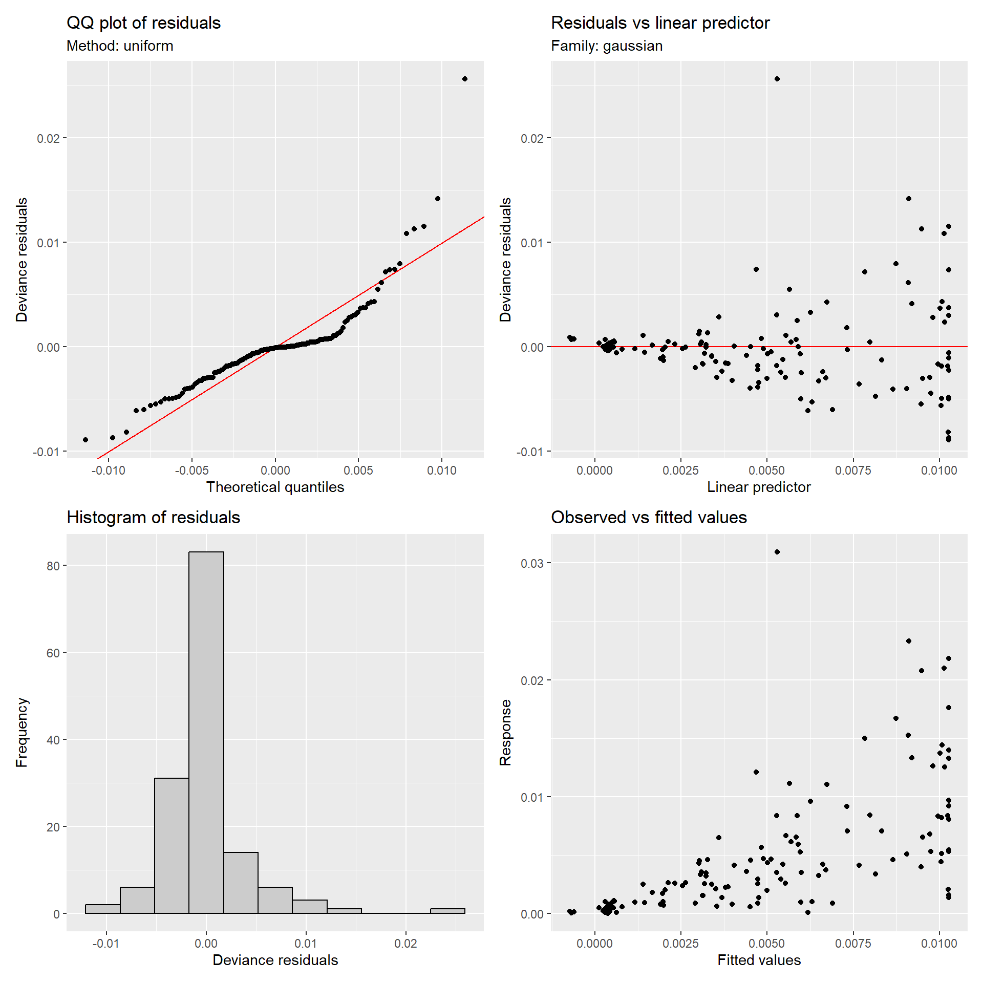
図2.24: Model diagnosis of M2_7
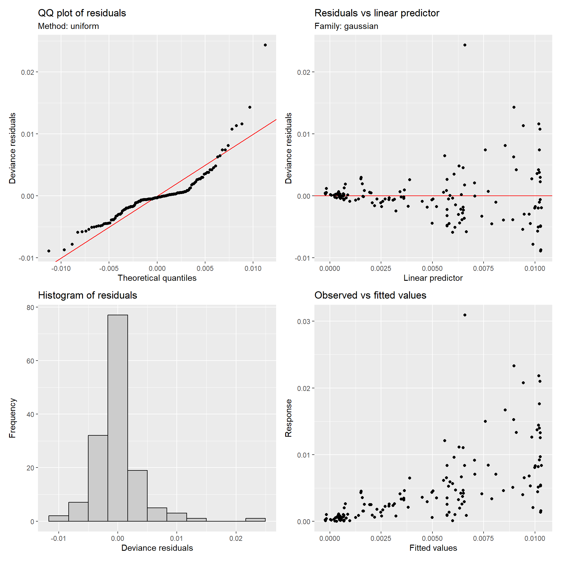
図2.25: Model diagnosis of M2_8
2.7 Transforming the density data
まず、魚の密度の平方根を目的変数とするように変数変換を行ったモデルを考える。
fish <- fish %>% mutate(Dens_sqrt = sqrt(Dens))

M2_9_a <- gam(Dens_sqrt ~ s(MeanDepth, by = Period) + Period, data = fish)
しかし、変数変換を施しても等分散性の仮定は両期間で満たされない。
data.frame(res = resid(M2_9_a),
           Period = fish$Period,
           MeanDepth = fish$MeanDepth) %>%
  ggplot(aes(x = MeanDepth, y = res))+
  geom_point(aes(fill = Period),
             shape = 21)+
  geom_hline(aes(yintercept = 0))+
  scale_fill_manual(values = c("white","black"))+
  theme_bw()+
  theme(aspect.ratio = 1)+
  labs(x = "Depth", y = "Residuals")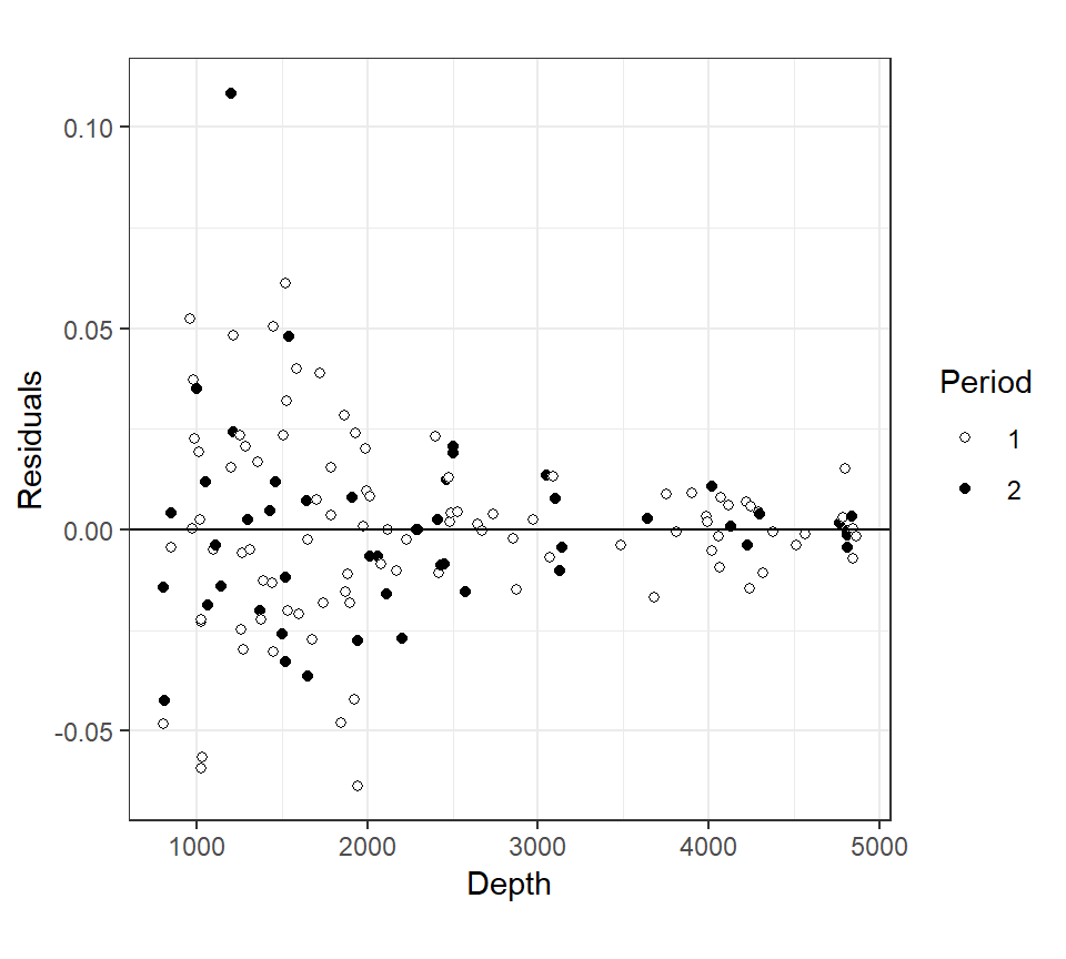
図2.26: Residuals versus Mean Depth for M2_9_a
魚の密度を対数変換することもできる。
fish <- mutate(fish, Dens_log = log(Dens))

M2_9_b <- gam(Dens_log ~ s(MeanDepth, by = Period) + Period, data = fish)
そうすると、等分散性の問題が解決されたように見える。
data.frame(res = resid(M2_9_b),
           Period = fish$Period,
           MeanDepth = fish$MeanDepth) %>%
  ggplot(aes(x = MeanDepth, y = res))+
  geom_point(aes(fill = Period),
             shape = 21)+
  geom_hline(aes(yintercept = 0))+
  scale_fill_manual(values = c("white","black"))+
  theme_bw()+
  theme(aspect.ratio = 1)+
  labs(x = "Depth", y = "Residuals")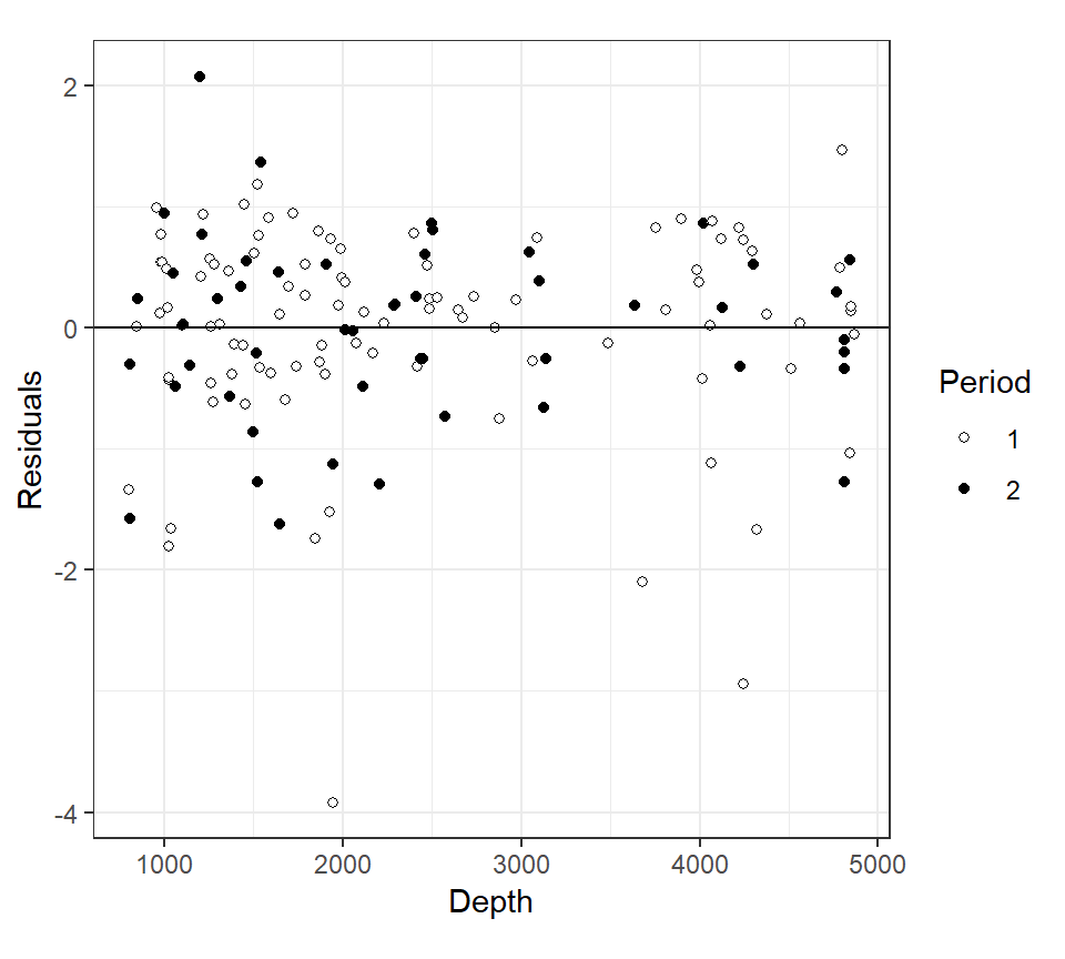
図2.27: Residuals versus Mean Depth for M2_9_b
ただし、QQプロットを見ると正規性の仮定は満たされていなさそう?
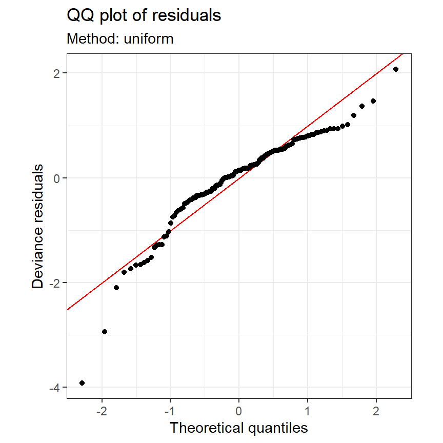
図2.28: QQplot for M2_9
2.8 Allowing for heterogeneity
変数変換の問題点は、大きい目的変数の方が小さいものよりもより圧縮されることで、期間ごとの違いが小さくなってしまう傾向があることである。 Pinheiro and Bates (2000) は、モデルの中に分散の不均等性を入れ込むことができることを示した。残差が従う正規分布の分散として\(\sigma^2\)ではなく、以下の3つのうちのいずれかを考える。
1つ目は、例えば期間ごと(\(s = 1, 2\))に異なる分散を考えるというものである。より細かくエリアごとに分散を求めたり、水深をカテゴライズしてそれぞれのカテゴリに異なる分散を割り当てることもできる。
2つ目と3つ目は、深さによって分散の値を変化させるというもので、その変化の仕方は最尤推定法によって推定されるパラメータ\(\delta\)によって決定される。
\[ \begin{aligned} \epsilon_i &\sim N(0, \sigma_s^2)\\ \epsilon_i &\sim N(0, \sigma^2 \times |Depth_i|^{2 \times \delta}) \\ \epsilon_i &\sim N(0, e^{2 \times \delta \times Depth_i}) \end{aligned} \tag{2.2} \]
Zuur (2009) は、正しい分散構造や共変量を選ぶための10ステップのプロトコルを書いている。1つの選択肢は、たくさんの分散構造のモデルを当てはめてみて、AICなどでモデル選択を行うというものである。もう一つは、通常の分散を持つモデルの残差からどのような分散構造を当てはめるべきかを検討するというものである。
2つ目のアプローチをとるとすると、図2.26は2通りに解釈できる。
- 水深が2000m以下のデータはそれ以外のデータより大きな分散をとる
- 水深が深くなるほど、分散は小さくなっていく
1つ目の解釈に従うとすると、残差の従う正規分布の分散は以下のように書ける。 \[ \begin{aligned} var(\epsilon_i) = \begin{cases} \sigma_2^2 & (Depth_i < 2000m)\\ \sigma_1^2 & (Depth_i > 2000m)\\ \end{cases} \end{aligned} \tag{2.3} \]
2つ目の解釈に従うとすると、式(2.2)の2つ目か3つ目のアプローチをとることになる。2つで推定される結果の違いはほとんどなく、問題になるのは\(Depth\)が0になるときだけであるが、今回は問題ない(\(Depth > 800\))。
式(2.3)はRでは以下のように実行できる。
fish %>%
  mutate(IMD = ifelse(MeanDepth < 2000, "1","2")) %>%
  mutate(IMD = as.factor(IMD)) -> fish

M2_10 <- mgcv::gamm(Dens ~ s(MeanDepth, by = Period) + Period,
              weights = varIdent(form =~ 1|IMD),
data = fish)結果は、M2_10$lmeとM2_10$gamの2つに格納されている(正直、lmeの方はよくわからない)。
summary(M2_10$lme)のVariance functionで推定されている1.000…と0.134…は、期間1と2の標準偏差(\(\sigma_1, \sigma_2\))がそれぞれ\(1.00 \times \sigma\)と\(0.13 \times \sigma\)であることを示している。\(\sigma\)の推定値はM2_10$lme$sigmaで求められ、0.0059であることから、期間1と2の分散はそれぞれ\((1.00 \times 0.0059)^2\)、\((0.13 \times 0.0059)^2\)である。
## Linear mixed-effects model fit by maximum likelihood
##   Data: strip.offset(mf)
##         AIC       BIC   logLik
##   -1354.792 -1330.869 685.3962
##
## Random effects:
##  Formula: ~Xr - 1 | g
##  Structure: pdIdnot
##                Xr1        Xr2        Xr3        Xr4        Xr5        Xr6
## StdDev: 0.00278938 0.00278938 0.00278938 0.00278938 0.00278938 0.00278938
##                Xr7        Xr8
## StdDev: 0.00278938 0.00278938
##
##  Formula: ~Xr.0 - 1 | g.0 %in% g
##  Structure: pdIdnot
##                Xr.01        Xr.02        Xr.03        Xr.04        Xr.05
## StdDev: 9.208057e-08 9.208057e-08 9.208057e-08 9.208057e-08 9.208057e-08
##                Xr.06        Xr.07        Xr.08    Residual
## StdDev: 9.208057e-08 9.208057e-08 9.208057e-08 0.005961115
##
## Variance function:
##  Structure: Different standard deviations per stratum
##  Formula: ~1 | IMD
##  Parameter estimates:
##         1         2
## 1.0000000 0.1348403
## Fixed effects:  y ~ X - 1
##                                 Value    Std.Error  DF   t-value p-value
## X(Intercept)              0.004957091 0.0003399765 143 14.580687  0.0000
## XPeriod2                 -0.002669103 0.0003924738 143 -6.800718  0.0000
## Xs(MeanDepth):Period1Fx1 -0.003085801 0.0011260515 143 -2.740373  0.0069
## Xs(MeanDepth):Period2Fx1 -0.001177319 0.0001825878 143 -6.447962  0.0000
##  Correlation:
##                          X(Int) XPerd2 X(MD):P1
## XPeriod2                 -0.866
## Xs(MeanDepth):Period1Fx1 -0.444  0.385
## Xs(MeanDepth):Period2Fx1  0.000 -0.313  0.000
##
## Standardized Within-Group Residuals:
##         Min          Q1         Med          Q3         Max
## -2.35949767 -0.40177858 -0.04041883  0.43543146  4.61217288
##
## Number of Observations: 147
## Number of Groups:
##          g g.0 %in% g
## 1 1##
## Family: gaussian
## Link function: identity
##
## Formula:
## Dens ~ s(MeanDepth, by = Period) + Period
##
## Parametric coefficients:
## Estimate Std. Error t value Pr(>|t|)
## (Intercept) 0.0049571 0.0003376 14.682 < 2e-16 ***
## Period2 -0.0026691 0.0003898 -6.848 2.14e-10 ***
## ---
## Signif. codes: 0 '***' 0.001 '**' 0.01 '*' 0.05 '.' 0.1 ' ' 1
##
## Approximate significance of smooth terms:
## edf Ref.df F p-value
## s(MeanDepth):Period1 3.388 3.388 68.42 <2e-16 ***
## s(MeanDepth):Period2 1.000 1.000 42.16 <2e-16 ***
## ---
## Signif. codes: 0 '***' 0.001 '**' 0.01 '*' 0.05 '.' 0.1 ' ' 1
##
## R-sq.(adj) = 0.62
## Scale est. = 3.5535e-05 n = 147図2.29は標準化残差とモデルからの予測値をプロットしたものである。標準化残差\(e_i^s\)は以下のように求められる。\(\sigma_j\)は期間ごとの分散である。プロットから、パターンが消えていることが確認できる。
\[ \begin{aligned} e_i &= Dens_i - \hat{\alpha} - \hat{f_1}(Depth_i) -\hat{f_2}(Depth_i) -\hat{\beta} \times Period_i \\ \epsilon_i^s &= \frac{e_i}{\sqrt{\hat{\sigma_j}^2}} \end{aligned} \]
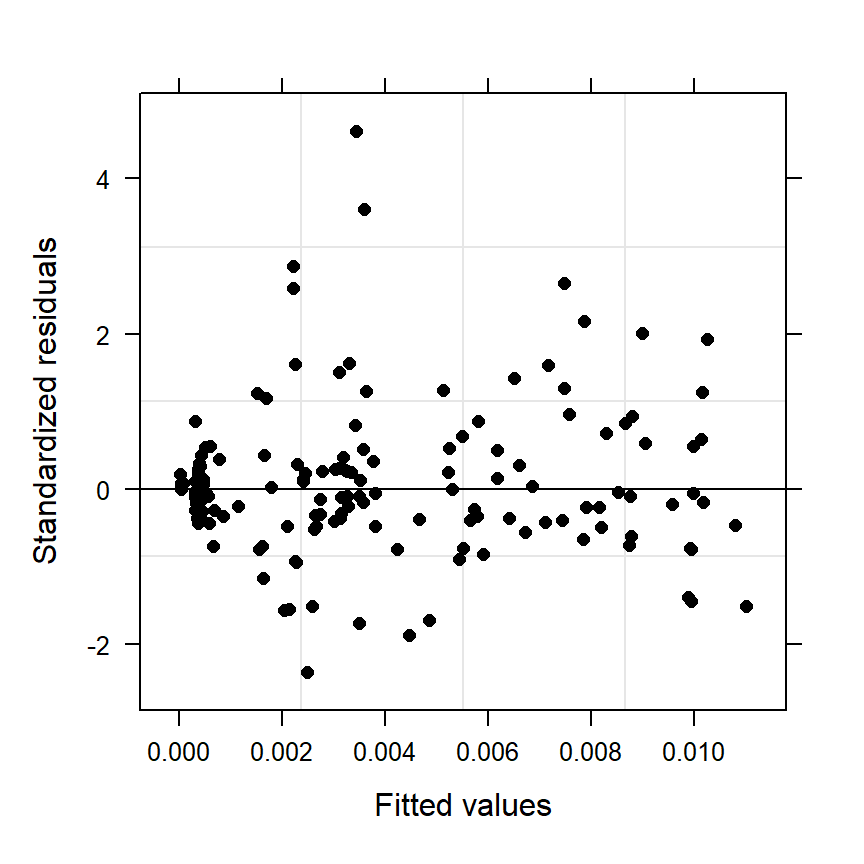
図2.29: Standardised residuals plotted versus fitted values obtained by the GAMM containing the varIdent residual variance structure.
ただし、QQプロットを見ると正規性の仮定は満たされていなさそう?
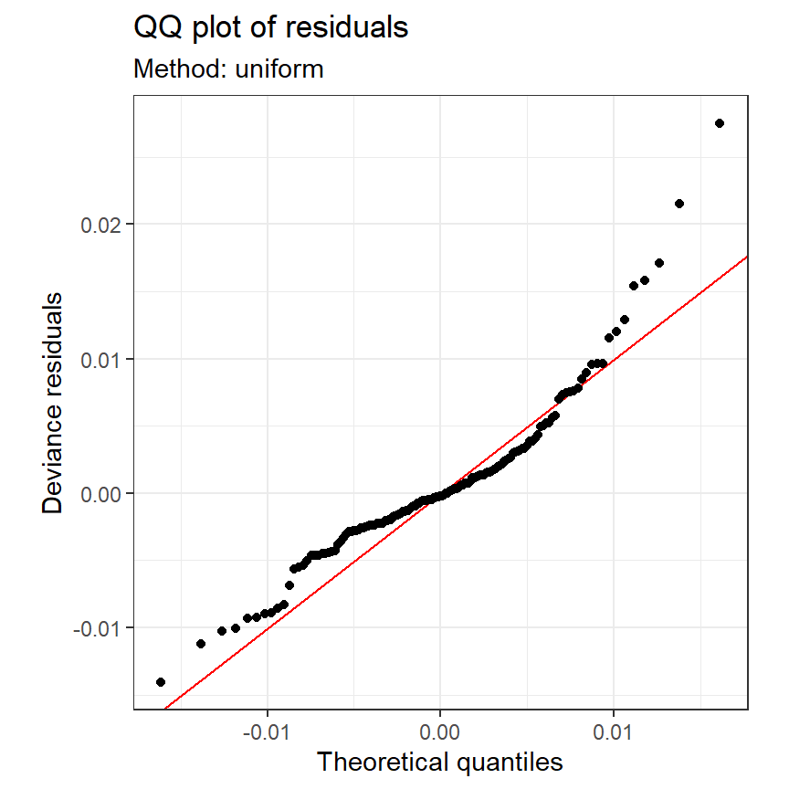
図2.30: QQplot for M2_10
2.9 Transforming and allowing for heterogeinity
変数変換を行ったうえでまた等分散性の仮定が満たされない場合は、加えて式(2.2)のいずれかの方法で分散を調整することもできる。 Bailey et al. (2009) では以下のモデルを適用している。
\[ \begin{aligned} \sqrt{Dens_i} &= \alpha + f(Depth_i) +f_2(Depth_i) + \epsilon_i \\ \epsilon_i &\sim N(0,\sigma_j^2)\\ \sigma^2_j &= \begin{cases} \sigma_2^2 & (Depth_i < 2000m)\\ \sigma_1^2 & (Depth_i > 2000m)\\ \end{cases} \\ \end{aligned} \]
Rでは以下のように実行できる。
M2_11 <- gamm(Dens_sqrt ~ s(MeanDepth, by = Period) + Period,
              weights = varIdent(form =~ 1|IMD),
data = fish)モデル診断を実行すると、等分散性の問題も正規性の問題も解決できているように見える(図2.31)。
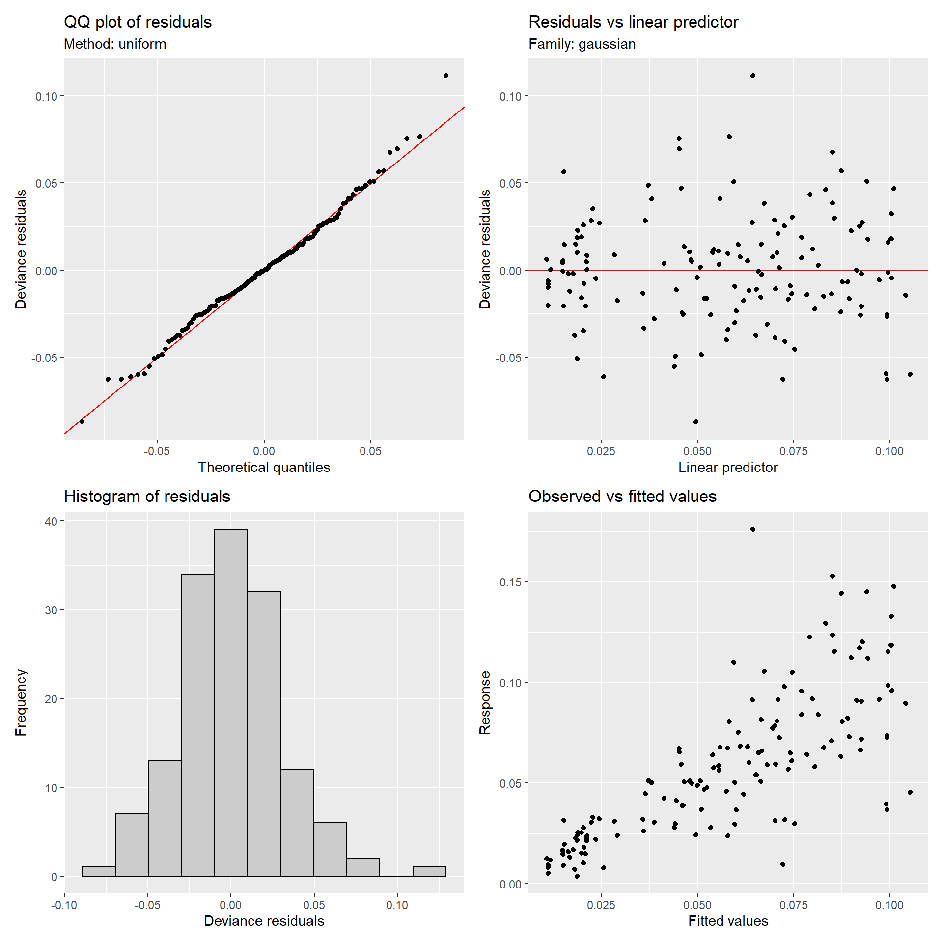
図2.31: Model diagnosis for M_11
モデルM2_7, M2_9_a、M2_9_b、M2_11から得られた平滑化曲線を図示したのが図2.32である。
fish %>%
  pivot_longer(cols = c(Dens,Dens_sqrt,Dens_log),
               values_to = "Dens", names_to = "type") %>%
  mutate(type = ifelse(str_detect(type,"sqrt"),"B",
                       ifelse(str_detect(type,"log"),"C","A"))) %>%
  bind_rows(fish %>% select(-Dens,-Dens_log) %>% rename(Dens = Dens_sqrt) %>% mutate(type = "D")) %>%
  mutate(Period = str_c("Period ",Period))-> fish_long


fitted_values(M2_7, data = nd, scale = "response") %>%
  mutate(type = "A") %>%
  bind_rows(fitted_values(M2_9_a, data = nd, scale = "response") %>%
              mutate(type = "B")) %>%
  bind_rows(fitted_values(M2_9_b, data = nd, scale = "response") %>%
              mutate(type = "C")) %>%
  bind_rows(fitted_values(M2_11, data = nd, scale = "response") %>%
              mutate(type = "D")) %>%
  mutate(Period = str_c("Period ", Period)) %>%
  ggplot(aes(x = MeanDepth))+
  geom_point(data = fish_long,
             aes(y = Dens, fill = Period),
             shape = 21, alpha = 0.7, size = 2.5)+
  scale_fill_manual(values = c("white","black"))+
  new_scale_fill()+
  geom_line(aes(y = fitted, linetype = Period),
            linewidth = 1.2)+
  geom_ribbon(aes(ymin = lower, ymax = upper, fill = Period),
              alpha = 0.3)+
  scale_fill_manual(values = c("grey45","red3"))+
  theme_bw(base_size = 13)+
  theme(aspect.ratio = 1,
        strip.text = element_text(hjust = 0),
        strip.background = element_blank())+
  labs(x = "Depth", y = expression(paste("Fish density")),
       fill = "Period", linetype = "Period")+
  guides(fill = guide_legend(override.aes = list(size = 3)))+
  facet_rep_wrap(~type, repeat.tick.labels = TRUE,
                 scales = "free_y")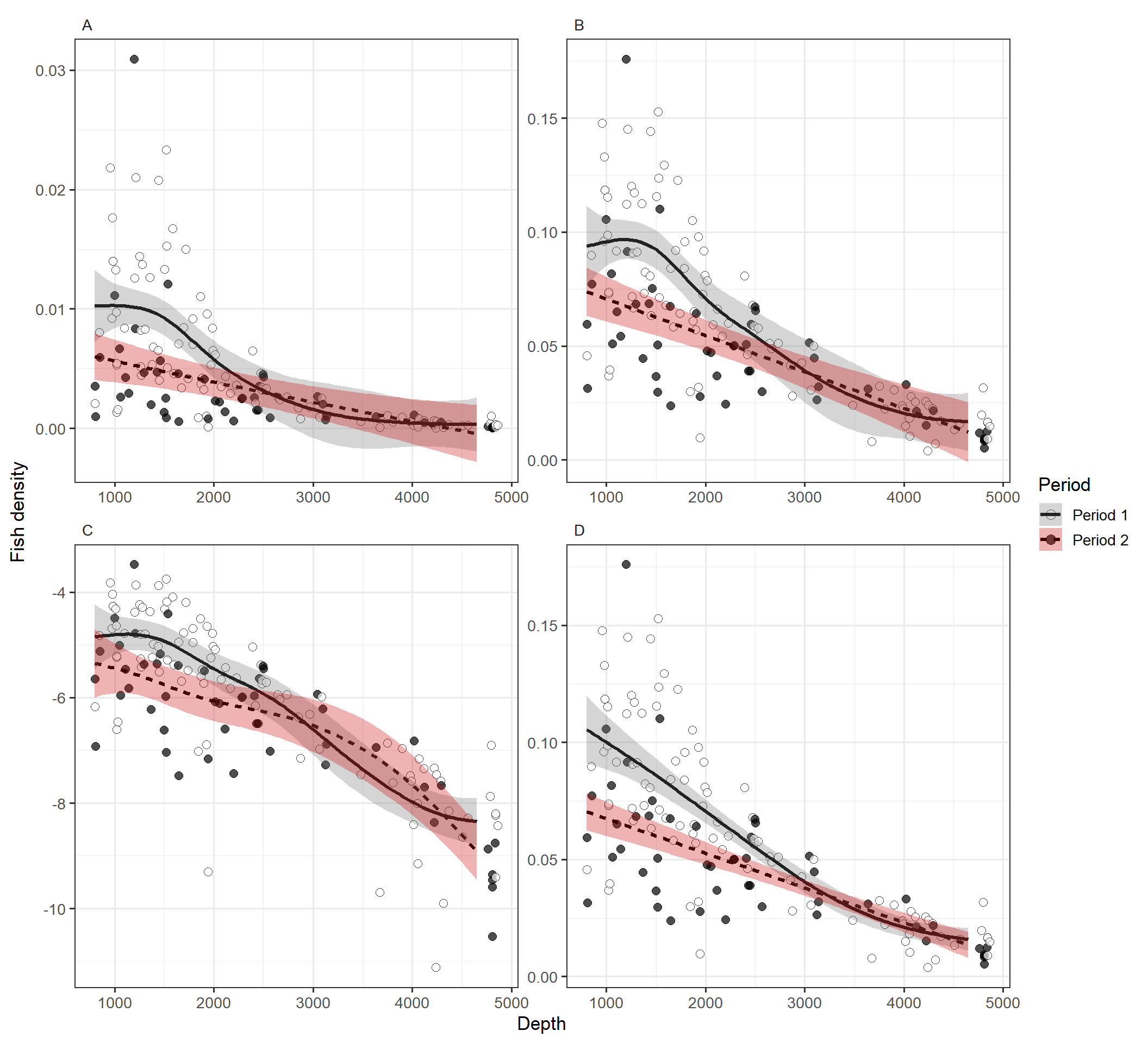
図2.32: Estimated smoothing curves obtained by a GAM. A: Gaussian GAM, B: Gaussian GAM square root density, C: Gaussian GAM log density, D: Gaussian GAM square root density, varIdent