3 Technical aspects of GAM using pelagic bioluminescent organisms
本章では、GAMの技術的な側面について説明を行う。
3.1 Pelagic bioluminescent organism data
GAMの技術的な側面を解説するため、本章では Heger et al. (2008) が2004年夏に海洋生物の発光について調べた研究を用いる。船で海洋を航行中に検出した蛍光の強度(Source)と、水深(Depth)、温度(Temp)、塩分(Salinity)、酸素(Oxgen)などを測定している。
データは14のステーションでサンプルされている。データは以下の通り。
BL <- read_delim("data/HegerPierce.txt")

datatable(BL,
          options = list(scrollX = 20),
          filter = "top")
3.2 Lineaar regression
まずは線形回帰を行う。ひとまず、ステーションの違いは無視して分析を行う。
図3.1は水深(Depth)と\(1m^3\)あたりに確認した生物発光の数をプロットしたものである。データを見る限り直線的な関係があるわけではないことが分かる。
BL %>%
  ggplot(aes(x = Depth, y = Sources)) +
  geom_point()+
  theme_bw(base_size = 12)+
  theme(aspect.ratio = 1)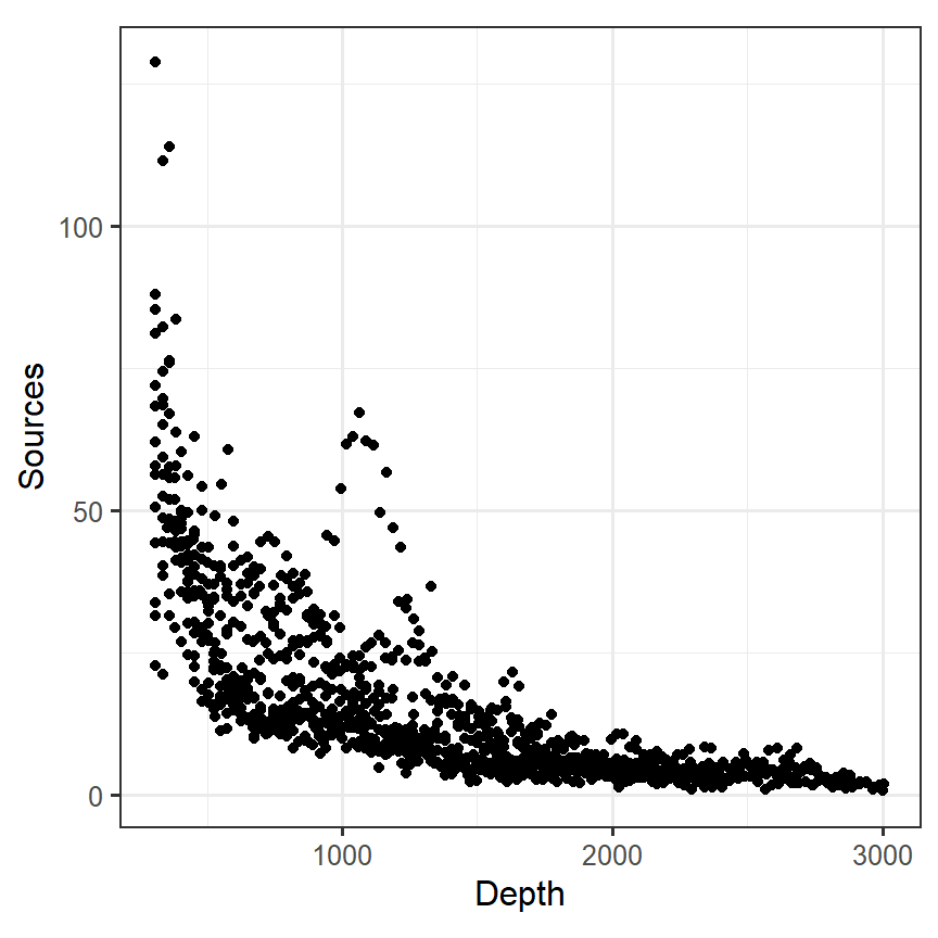
図3.1: Scatterplot of depth versus bioluminescence sources per m^3
以下のモデリングでは、水深を0から1にスケーリングする(モデルがうまく回らなくなるため)。
明確に直線的な関係はないが、まずは線形回帰を行う。データには様々な変数があるが、いくつかの変数は強く相関しているため、水深のみを説明変数として用いる(図3.2)。
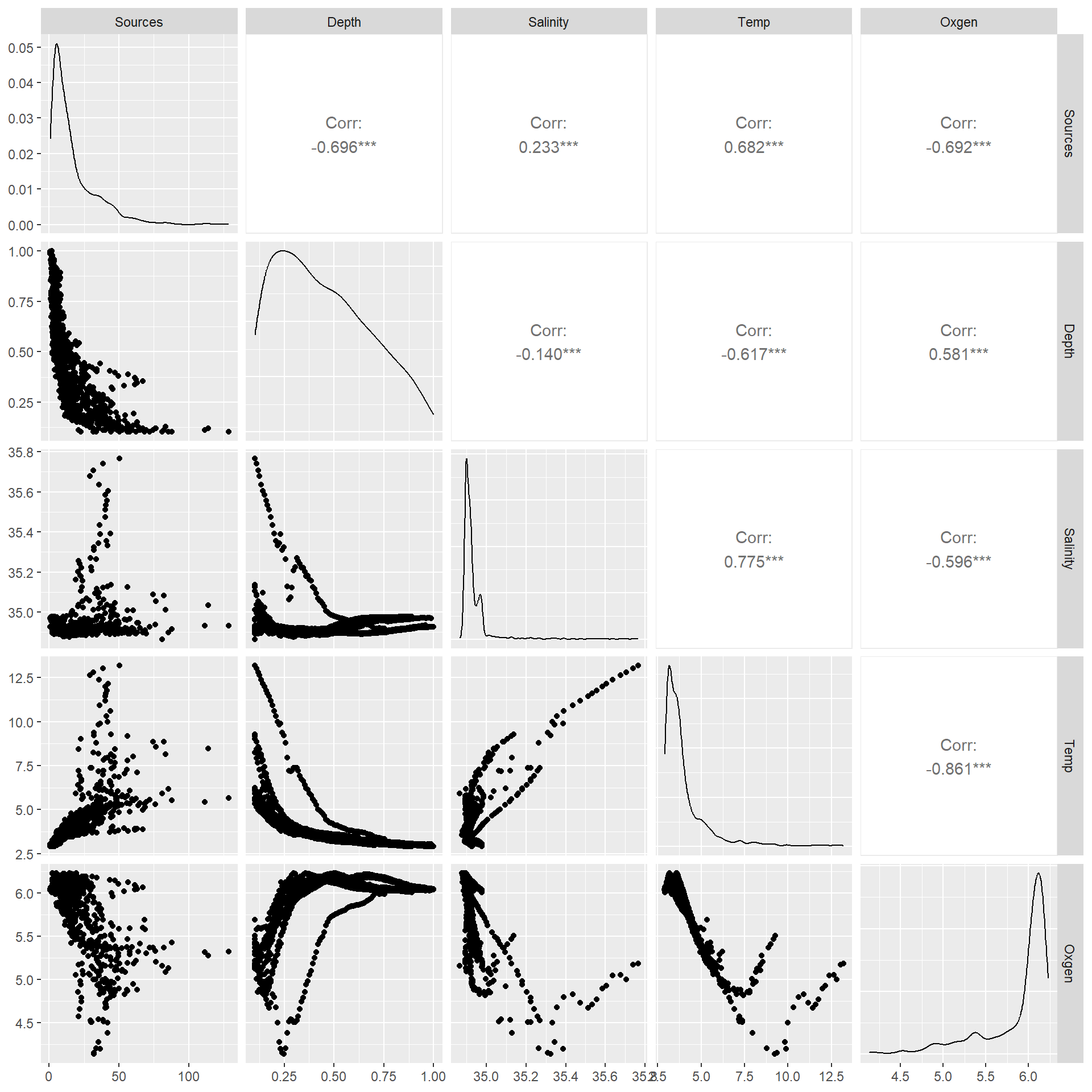
図3.2: Pair plot of the data.
モデル式は以下のようになる。
\[
\begin{aligned}
Sources_i &= \alpha + \beta \times Depth_i + \epsilon_i\\
\epsilon_i &\sim N(0, \sigma^2)
\end{aligned}
\]
Rでは以下のように実行する。
モデルによって推定された回帰直線をデータに当てはめると、明らかに当てはまりが悪いことが分かる(図3.3)。
nd_M3 <- data.frame(Depth = seq(0,1,length.out = 100))

fitted_M3_1 <- predict(M3_1, newdata = nd_M3) %>%
  data.frame() %>%
  rename(fitted = 1) %>%
  bind_cols(nd_M3)

BL %>%
  ggplot(aes(x = Depth, y = Sources))+
  geom_point(size = 2, alpha = 0.6, color = "grey54")+
   geom_line(data = fitted_M3_1,
            aes(y = fitted),
            linewidth = 1)+
  theme_bw(base_size = 12)+
  theme(aspect.ratio = 1)+
  coord_cartesian(ylim = c(0,120))+
  labs(x = "Scaled depth", y = "Sources")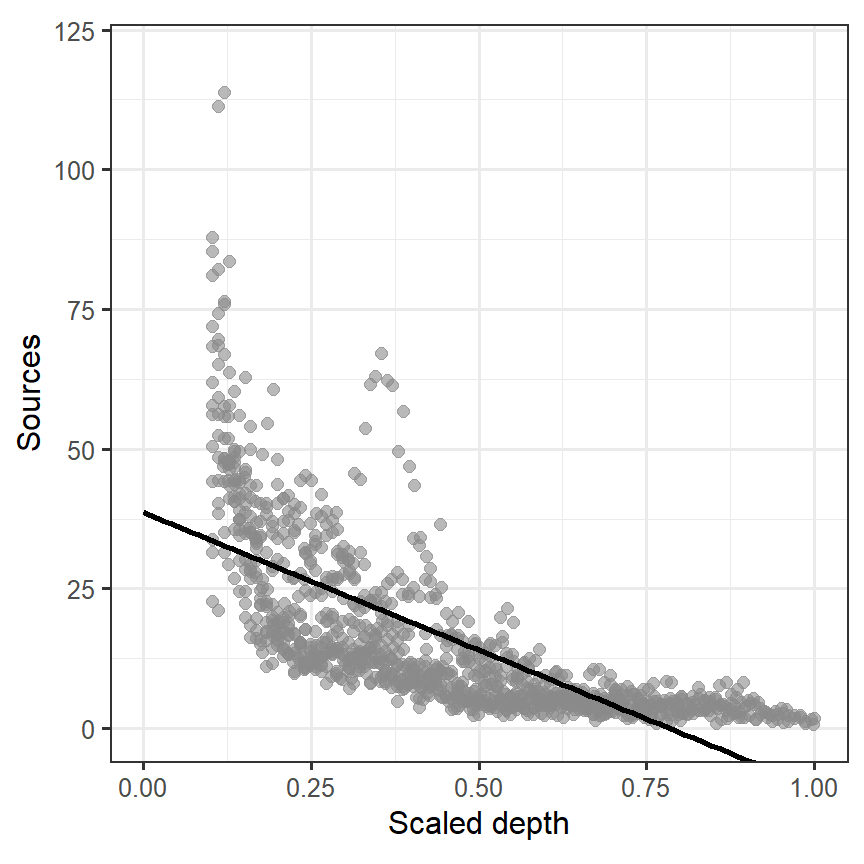
図3.3: Fitted line estimated from M3_1
本章の目的は、以下のような式を書いたときに\(Depth\)と\(Sources\)の関係をうまく説明できる\(f(Depth_i)\)という関数を見つけることである。先ほどの線形回帰では\(f(Depth_i) = \beta \times Depth_i\)だった。次節以降では、\(f(Depth_i)\)として何が最適かを探っていき、最終的にGAMの解説を行う。
\[ Sources_i = \alpha + f(Depth_i) + \epsilon_i \tag{3.1} \]
3.3 Polynomial regression model
続いて、多項式回帰を行ってみる。モデル式は以下のとおりである。
\[ \begin{aligned} Sources_i &= \alpha + \beta_1 \times Depth_i + \beta_2 \times Depth_i^2 + \beta_3 \times Depth^3 + \epsilon_i\\ \epsilon_i &\sim N(0, \sigma^2) \end{aligned} \]
Rでは以下のコードで実行できる。
モデルによって推定された曲線をデータの上に描いたのが図3.4である。先ほどよりは当てはまりがよくなったが、左上と右下の当てはまりが悪いことが分かる。
fitted_M3_2 <- predict(M3_2, newdata = nd_M3,) %>%
  data.frame() %>%
  rename(fitted = 1) %>%
  bind_cols(nd_M3)

BL %>%
  ggplot(aes(x = Depth, y = Sources))+
  geom_point(size = 2, alpha = 0.6, color = "grey54")+
   geom_line(data = fitted_M3_2,
            aes(y = fitted),
            linewidth = 1)+
  theme_bw(base_size = 12)+
  theme(aspect.ratio = 1)+
  coord_cartesian(ylim = c(0,120), xlim = c(0.1,1))+
  labs(x = "Scaled depth", y = "Sources")
図3.4: Fitted line estimated from M3_2
次節からは、GAMの数理的な基礎を理解するためにも以下を解説する。
- 線形スプライン回帰(linear spline regression)
- 二次スプライン回帰(quadratic spline regression)
- ノット数(numer of knots)
- 罰則付きスプライン回帰(penalized spline regression)
3.4 Linear spline regression
線形スプライン回帰とは、x軸をいくつかのセグメントに分け、それぞれのセグメントごとに線形回帰を行う方法である。問題は、いくつのセグメントにどのように分けるべきかということである。
図3.3や図3.4からは、スケール化された水深がだいたい0.2くらいで傾きが変わっている印象を受ける。そこで、0.2を境に傾きが変わるモデルを考える。ただし、このとき回帰直線は0.2でつながっていなければいけない。
実際にモデルを適用する前に、\((Depth_i - 0.2)_+\)を以下のように定義する。
\[ (Depth_i - 0.2)_+ = \begin{cases} 0 & (Depth_i < 0.2)\\ Depth_i - 0.2 & (Depth_i ≧ 0.2)\\ \end{cases} \]
Rでは以下のような関数rhsを作成してこうした変数を作成する。これは、ある変数xについて閾値THを境にそれ以下なら0、それ以上なら\(x - TH\)となるような新しい変数を作成する関数である。
モデルは以下のようになる。
\[
\begin{aligned}
Sources_i &= \alpha + \beta_1 \times Depth_i + \beta_{11} \times (Depth_i - 0.2)_+ + \epsilon_i \\
\epsilon_i &\sim N(0,\sigma^2)
\end{aligned}
\]
Rでこれを実装すると以下のようになる。
モデルから推定された回帰曲線は以下のようになる(図3.5)。
fitted_M3_3 <- predict(M3_3, newdata = nd_M3) %>%
  data.frame() %>%
  rename(fitted = 1) %>%
  bind_cols(nd_M3)

BL %>%
  ggplot(aes(x = Depth, y = Sources))+
  geom_point(size = 2, alpha = 0.6, color = "grey54")+
  geom_line(data = fitted_M3_3,
            aes(y = fitted),
            linewidth = 1)+
  theme_bw(base_size = 12)+
  theme(aspect.ratio = 1)+
  coord_cartesian(ylim = c(0,120), xlim = c(0.1,1))+
  labs(x = "Scaled depth", y = "Sources")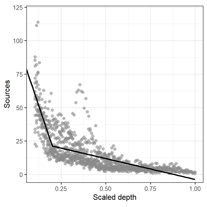
図3.5: Fitted line estimated from M3_3
問題は、モデルM3_3が通常の直線回帰モデル(M3_1)や多項回帰モデル(M3_2)よりもよいモデルかどうかである。赤池情報量規準(AIC)を持ちると3、M3_3はより予測の良いモデルだということが分かる。
しかし、モデルM3_3にも問題点がいくつかある。\(Depth = 0.2\)での傾きの変化が急激であるということと、0.2という数値の選択基準が恣意的である点である。
こうした問題点を解決する手段として、例えばデータを10等分してそれぞれについて回帰直線を当てはめるというようなものが考えられる。この場合、傾きは以下の9ポイント(第1から第9十分位数)で変わることになる。このようなポイントをノット(knot)という。
このとき、モデル式は以下のように書ける。なお、\(k_j\)は第j十分位数を表す。
\[ \begin{aligned} Sources_i &= \alpha + \beta_1 \times Depth_i + \sum_{j = 1}^9 \Bigl( \beta_{1j} \times (Depth_i - k_j)_+ \Bigl) + \epsilon_i \\ \epsilon_i &\sim N(0,\sigma^2) \end{aligned} \]
このモデルはRで以下のように実装できる。
M3_4 <- lm(Sources ~ Depth + rhs(Depth, q_Depth[1]) + rhs(Depth, q_Depth[2]) +
             rhs(Depth, q_Depth[3]) + rhs(Depth, q_Depth[4]) + rhs(Depth, q_Depth[5]) +
             rhs(Depth, q_Depth[6]) + rhs(Depth, q_Depth[7]) + rhs(Depth, q_Depth[8]) +
rhs(Depth, q_Depth[9]), data = BL)このモデルによって推定された回帰曲線は以下のとおりである(図3.6)。
fitted_M3_4 <- predict(M3_4, newdata = nd_M3) %>%
  data.frame() %>%
  rename(fitted = 1) %>%
  bind_cols(nd_M3)

BL %>%
  ggplot(aes(x = Depth, y = Sources))+
  geom_point(size = 2, alpha = 0.6, color = "grey54")+
  geom_line(data = fitted_M3_4,
            aes(y = fitted),
            linewidth = 1)+
  theme_bw(base_size = 12)+
  theme(aspect.ratio = 1)+
  coord_cartesian(ylim = c(0,120), xlim = c(0.1,1))+
  labs(x = "Scaled depth", y = "Sources")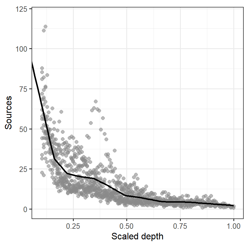
図3.6: Fitted line estimated from M3_4
先ほどよりもよりデータへの当てはまりはよくなっているが、まだカクカクした線になっている。より細かく\(Depth\)を区分することは可能である。
model.matrix(M3_4)によって得られるこのモデルのsmootherの要素となった以下のものは、smootherの基底(smoother)と呼ばれる。
\[ 1, Depth_i, (Depth_i - k_1)_+, (Depth_i - k_2)_+, \dots, (Depth_i - k_9)_+ \]
3.5 Quadratic spline regression
適切な\(f(Depth_i)\)を探す試みとして線形スプライン回帰を行ったが、ノットで傾きがカクカクしてしまっていた。これに代わる方法として、二次スプライン回帰(quadratic spline regression)を考えることができる。モデルは以下のように書ける。
\[ \begin{aligned} Sources_i &= \alpha + \beta_1 \times Depth_i + \beta_2 \times Depth_i^2 + \sum_{j = 1}^k \Bigl( \beta_{1j} \times (Depth_i - k_j)_+^2 \Bigl) + \epsilon_i \\ \epsilon_i &\sim N(0,\sigma^2) \end{aligned} \tag{3.2} \]
そのため、\(Depth_i\)を10等分するのであれば、このモデルにおける基底は以下の12個になる。
\[
1, Depth_i^2, (Depth_i - k_1)_+^2, (Depth_i - k_2)_+^2, \dots, (Depth_i - k_9)_+^2
\]
このモデルをRで実装するため、以下の関数を作成する。これは、ある変数xについて閾値THを境にそれ以下なら0、それ以上なら\((x - TH)^2\)となるような新しい変数を作成する関数である。
モデルは以下のように実行できる。
M3_5 <- lm(Sources ~ Depth + I(Depth^2) + rhs2(Depth, q_Depth[1]) + rhs2(Depth, q_Depth[2]) +
             rhs2(Depth, q_Depth[3]) + rhs2(Depth, q_Depth[4]) + rhs2(Depth, q_Depth[5]) +
             rhs2(Depth, q_Depth[6]) + rhs2(Depth, q_Depth[7]) + rhs2(Depth, q_Depth[8]) +
rhs2(Depth, q_Depth[9]), data = BL)このモデルによって推定された回帰曲線は以下のとおりである(図3.7)。線形スプライン回帰よりもなめらかな曲線になっていることが分かる。
fitted_M3_5 <- predict(M3_5, newdata = nd_M3) %>%
  data.frame() %>%
  rename(fitted = 1) %>%
  bind_cols(nd_M3)

BL %>%
  ggplot(aes(x = Depth, y = Sources))+
  geom_point(size = 2, alpha = 0.6, color = "grey54")+
  geom_line(data = fitted_M3_5,
            aes(y = fitted),
            linewidth = 1)+
  theme_bw(base_size = 12)+
  theme(aspect.ratio = 1)+
  coord_cartesian(ylim = c(0,120), xlim = c(0.1,1))+
  labs(x = "Scaled depth", y = "Sources")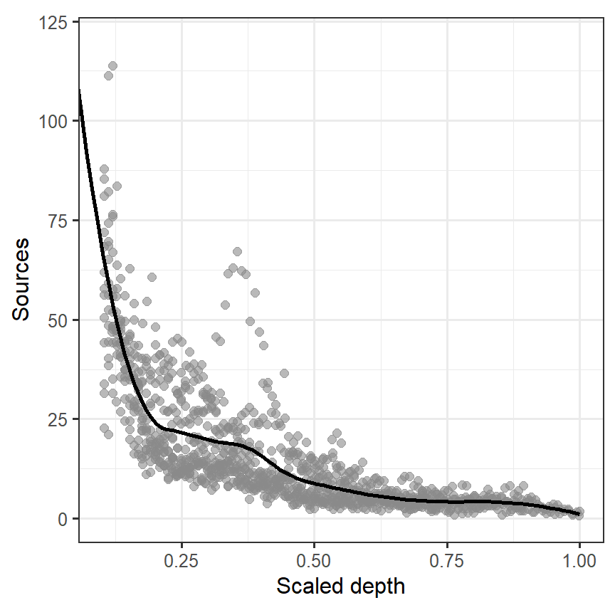
図3.7: Fitted line estimated from M3_5
以下、モデルの結果を見てみよう。rhs2関数で作られた変数の多くが有意でないのは、これらが強く相関しており多重共線性の問題があることが原因だろう。
##
## Call:
## lm(formula = Sources ~ Depth + I(Depth^2) + rhs2(Depth, q_Depth[1]) +
##     rhs2(Depth, q_Depth[2]) + rhs2(Depth, q_Depth[3]) + rhs2(Depth,
##     q_Depth[4]) + rhs2(Depth, q_Depth[5]) + rhs2(Depth, q_Depth[6]) +
##     rhs2(Depth, q_Depth[7]) + rhs2(Depth, q_Depth[8]) + rhs2(Depth,
##     q_Depth[9]), data = BL)
##
## Residuals:
##     Min      1Q  Median      3Q     Max
## -42.285  -4.850  -1.006   2.705  63.710
##
## Coefficients:
##                          Estimate Std. Error t value Pr(>|t|)
## (Intercept)               175.444     28.621   6.130 1.25e-09 ***
## Depth                   -1410.486    409.840  -3.442 0.000601 ***
## I(Depth^2)               3291.466   1430.389   2.301 0.021584 *
## rhs2(Depth, q_Depth[1])  -549.110   2067.208  -0.266 0.790578
## rhs2(Depth, q_Depth[2]) -2891.946   1340.997  -2.157 0.031269 *
## rhs2(Depth, q_Depth[3])   368.134   1190.504   0.309 0.757212
## rhs2(Depth, q_Depth[4])  -935.978   1061.824  -0.881 0.378262
## rhs2(Depth, q_Depth[5])  1197.211    877.679   1.364 0.172843
## rhs2(Depth, q_Depth[6])  -445.930    730.756  -0.610 0.541842
## rhs2(Depth, q_Depth[7])    30.872    592.644   0.052 0.958466
## rhs2(Depth, q_Depth[8])     5.152    400.189   0.013 0.989732
## rhs2(Depth, q_Depth[9])  -152.712    295.507  -0.517 0.605421
## ---
## Signif. codes:  0 '***' 0.001 '**' 0.01 '*' 0.05 '.' 0.1 ' ' 1
##
## Residual standard error: 9.148 on 1037 degrees of freedom
## Multiple R-squared:  0.6892, Adjusted R-squared:  0.6859
## F-statistic: 209.1 on 11 and 1037 DF, p-value: < 2.2e-16式(3.2)のモデルは正規分布の一般化加法モデルといえる。mgvcパッケージではより発展的なsmootherを用いており、多重共線性の問題などが生じないようなっている。
このモデルは第1章のときのように以下のように書ける。なお、\(\mathbf{y}\)は目的変数をすべて含むベクトル、\(\mathbf{X}\)はmodel.matrix(M3_5)によって得られる基底の行列、\(\mathbf{\beta}\)は回帰係数をすべて含むベクトルである。この表現で書けるということは、第1章と全く同じ方法で標準誤差や自由度、信頼区間、予測区間を算出できるということである。
\[
\mathbf{y} = \mathbf{X} \times \mathbf{\beta} + \mathbf{\epsilon}
\]
3.6 Cubic regression splines
より回帰曲線を滑らかにするのであれば、3次スプライン回帰を考えることもできる。モデル式は以下の通り。Rでも前節までと同様に実行することができる。
\[ \begin{aligned} Sources_i &= \alpha + \beta_1 \times Depth_i + \beta_2 \times Depth_i^2 + \beta_3 \times Depth_i^3 + \sum_{j = 1}^k \Bigl( \beta_{1j} \times (Depth_i - k_j)_+^3 \Bigl) + \epsilon_i \\ \epsilon_i &\sim N(0,\sigma^2) \end{aligned} \tag{3.3} \]
Wood (2017) や Zuur (2009) では、さらに発展的な方法として以下のモデルを考えた。
\[ \begin{aligned} Sources_i &= \sum_{j = 1}^K \Bigl( \beta_{j} \times b_j(Depth_i) \Bigl) + \epsilon_i \\ \epsilon_i &\sim N(0,\sigma^2) \end{aligned} \tag{3.4} \]
ここで、\(b_1(Depth_i) = 1, b_2(Depth_i) = Depth\)であり、\(j ≧ 2\)のときは\(B_j(Depth_i) = R(Depth_i, k_{j-2})\)である。また、\(k_{j-2}\)は\(j-2\)番目のノットの値を表す。よって、以下のようにも書ける。
\[ \begin{aligned} Sources_i &= \beta_1 + \beta_1 \times Depth_i + \sum_{j = 2}^K \Bigl( \beta_{j} \times R(Depth_i, k_{j-2}) \Bigl) + \epsilon_i \\ \epsilon_i &\sim N(0,\sigma^2) \end{aligned} \tag{3.5} \]
なお、\((Depth_i, k_{j-2})\)は以下のように定義される。
\[ R(X,z) = \frac{1}{4} \times \Bigl( (z - \frac{1}{2})^2 - \frac{1}{12} \Bigl) \times \Bigl( (X - \frac{1}{2})^2 - \frac{1}{12} \Bigl) - \frac{1}{24} \times \Bigl( (|X-z| - \frac{1}{2})^4 - \frac{1}{2}(|X-z| - \frac{1}{2})^2 + \frac{7}{240} \Bigl) \]
Rでもこの関数を作成する。
rk <-function(x, z){
  ((z-0.5)^2-1/12)*((x-0.5)^2-1/12)/4 - ((abs(x-z)-0.5)^4-0.5*(abs(x-z)- 0.5)^2 +7/240)/24
}また、説明変数をすべて含む行列\(\mathbf{X}\)を作成する必要がある。この行列は1列目は全て1、2列目は\(Depth_i\)で、3列目以降は\(R(Depth_i, k_{j-2})\)である。Rでは以下のように作成できる。
spl.X <-function(x, xk){
  q <-length(xk) + 2
  n <-length(x)
  X <-matrix(1, n, q)
  X[,2] <-x
  X[,3:q] <-outer(x, xk, FUN = rk)
  X
}

X <- spl.X(BL$Depth, q_Depth)Rでモデルを以下のように実行できる。なお、\(\mathbf{X}\)にはすでに切片に相当する1列目が含まれているため、Sources ~ X - 1とする。
このモデルによって推定された回帰曲線は以下のとおりである(図3.8)。2次スプライン回帰の結果と大きくは違わない。
Xp <- spl.X(nd_M3$Depth, q_Depth)

fitted_M3_6 <- data.frame(Depth = nd_M3$Depth,
                          fitted = Xp %*% coef(M3_6))

BL %>%
  ggplot()+
  geom_point(aes(x = Depth, y = Sources),
             size = 2, alpha = 0.6, color = "grey54")+
  geom_line(data = fitted_M3_6,
            aes(x = Depth, y = fitted),
            linewidth = 1)+
  geom_vline(xintercept = q_Depth,
             linetype = "dashed")+
  theme_bw(base_size = 12)+
  theme(aspect.ratio = 1)+
  coord_cartesian(ylim = c(0,120), xlim = c(0.1,1))+
  labs(x = "Scaled depth", y = "Sources")
図3.8: Fitted line estimated from M3_6
3.7 The number of knots
第3.4から3.6節までは\(Depth_i\)を10の区間に分けており、両端を除くとノット数は9だった。しかし、この数はあくまでも恣意的に選択したものに過ぎない。それでは、私たちはノット数をいくつに設定するのが適切なのだろうか。
図3.9は両端を除くノット数を変化させたときの回帰曲線を図示したものである。結果を見てみると、ノット数による違いはそこまで大きくないように思える。
num <- c(1,3,5,7,9,11,13,15,17, 19, 31)
q_Depth_list <- list()
X_list <- list()

for(i in seq_along(num)){
q_Depth_list[[i]] <- quantile(BL$Depth, probs = seq(0,1,by = 1/(num[i]+1)))[2:(num[i]+1)]
X_list[[i]] <- spl.X(BL$Depth, q_Depth_list[[i]])
}

M3_6_list <- list()
Xp_list <- list()
fitted_list <- list()

for(i in seq_along(num)){
  M3_6_list[[i]] <- lm(Sources ~ X_list[[i]] - 1, data = BL)
  Xp_list[[i]] <- spl.X(nd_M3$Depth, q_Depth_list[[i]])
  fitted_list[[i]] <- data.frame(Depth = nd_M3$Depth,
                                 fitted = Xp_list[[i]] %*% coef(M3_6_list[[i]]),
                                 knot = num[i])
}

bind_rows(fitted_list[1], fitted_list[[2]], fitted_list[[3]], fitted_list[[4]],
          fitted_list[[5]], fitted_list[[6]], fitted_list[[7]], fitted_list[[8]],
          fitted_list[[9]], fitted_list[[10]], fitted_list[[11]]) %>%
  mutate(knot_text = str_c("inner knot = ", knot)) %>%
  mutate(knot_text = fct_reorder(knot_text, knot))-> fitted_all

BL %>%
  ggplot()+
  geom_point(aes(x = Depth, y = Sources),
             size = 2, alpha = 0.6, color = "grey54")+
  geom_line(data = fitted_all,
            aes(x = Depth, y = fitted),
            linewidth = 1)+
  facet_rep_wrap(~knot_text, repeat.tick.labels = TRUE)+
  theme_bw(base_size = 12)+
  theme(aspect.ratio = 1,
        strip.background = element_blank(),
        strip.text = element_text(hjust = 0))+
  coord_cartesian(ylim = c(0,120), xlim = c(0.105,1))+
  labs(x = "Scaled depth", y = "Sources")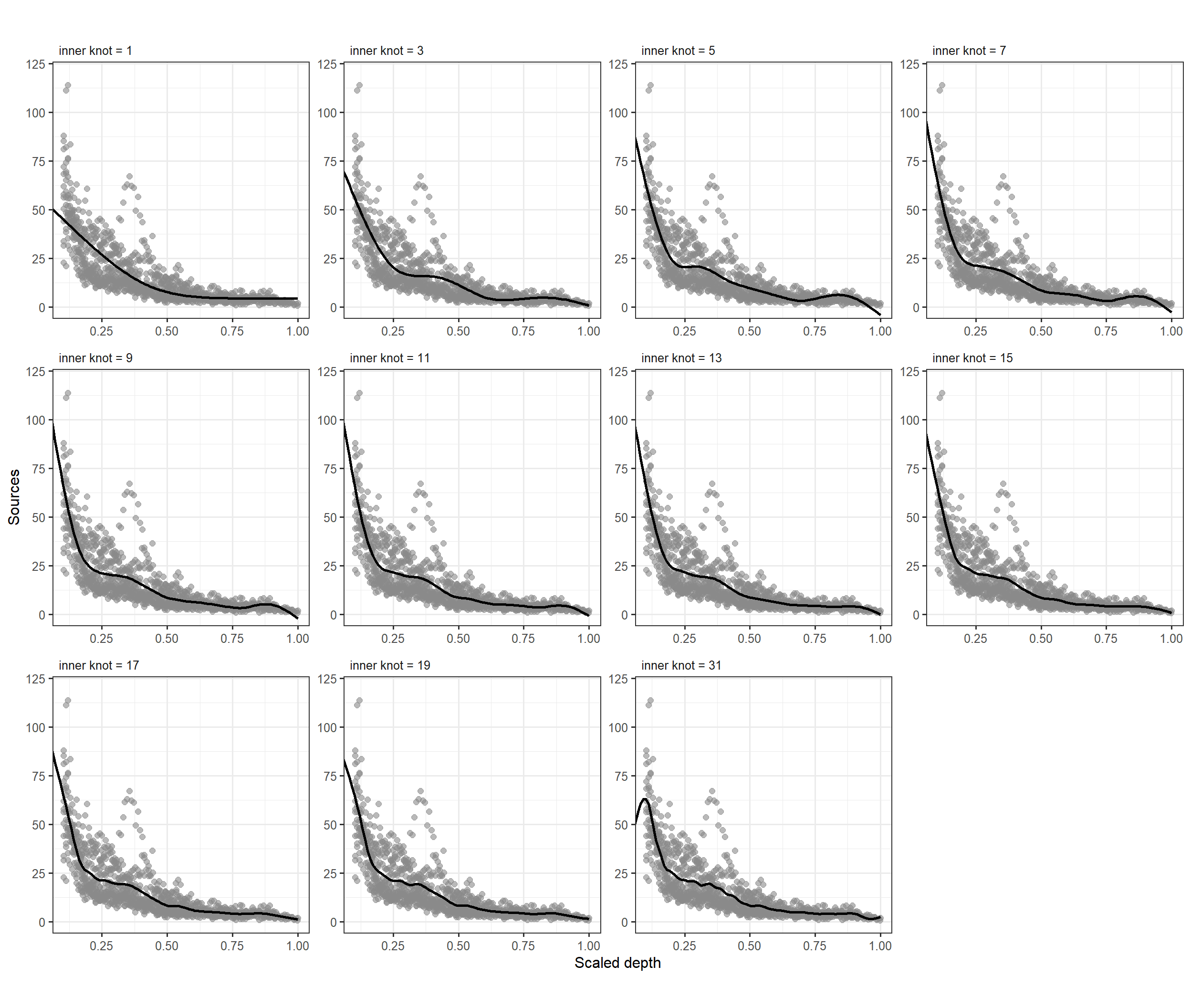
図3.9: Fitted smoothers for a quadratic spline regression model using different numbers of knots.
AICなどによってこれらのモデルの比較を行うことはできる(図3.10)。AICとAICcに基づくとノット数が7のモデルが最もよく(値が最も小さく)、そこからノット数が離れるほど予測がよくなくなる(= 値が大きくなる)。BICに基づくとノット数が5のときが最も予測が良い。
compare_performance(M3_6_list[[1]],M3_6_list[[2]],M3_6_list[[3]],
                    M3_6_list[[4]],M3_6_list[[5]],M3_6_list[[6]],
                    M3_6_list[[7]],M3_6_list[[8]],M3_6_list[[9]],
                    M3_6_list[[10]],M3_6_list[[11]]) %>%
  data.frame() %>%
  mutate(knot = num) %>%
  select(knot, AIC, AICc, BIC, R2, R2_adjusted) %>%
  pivot_longer(c(AIC, AICc, BIC), names_to = "IC", values_to = "value") %>%
  ggplot(aes(x = knot, y = value))+
  geom_point(aes(color = IC, shape = IC),
             size = 5, stroke = 2,
             alpha = 0.7)+
  scale_shape_manual(values = c(1,5,0))+
  scale_x_continuous(breaks = num)+
  labs(y = "Information criteria", color = "", shape = "")+
  theme_bw()+
  theme(aspect.ratio = 1)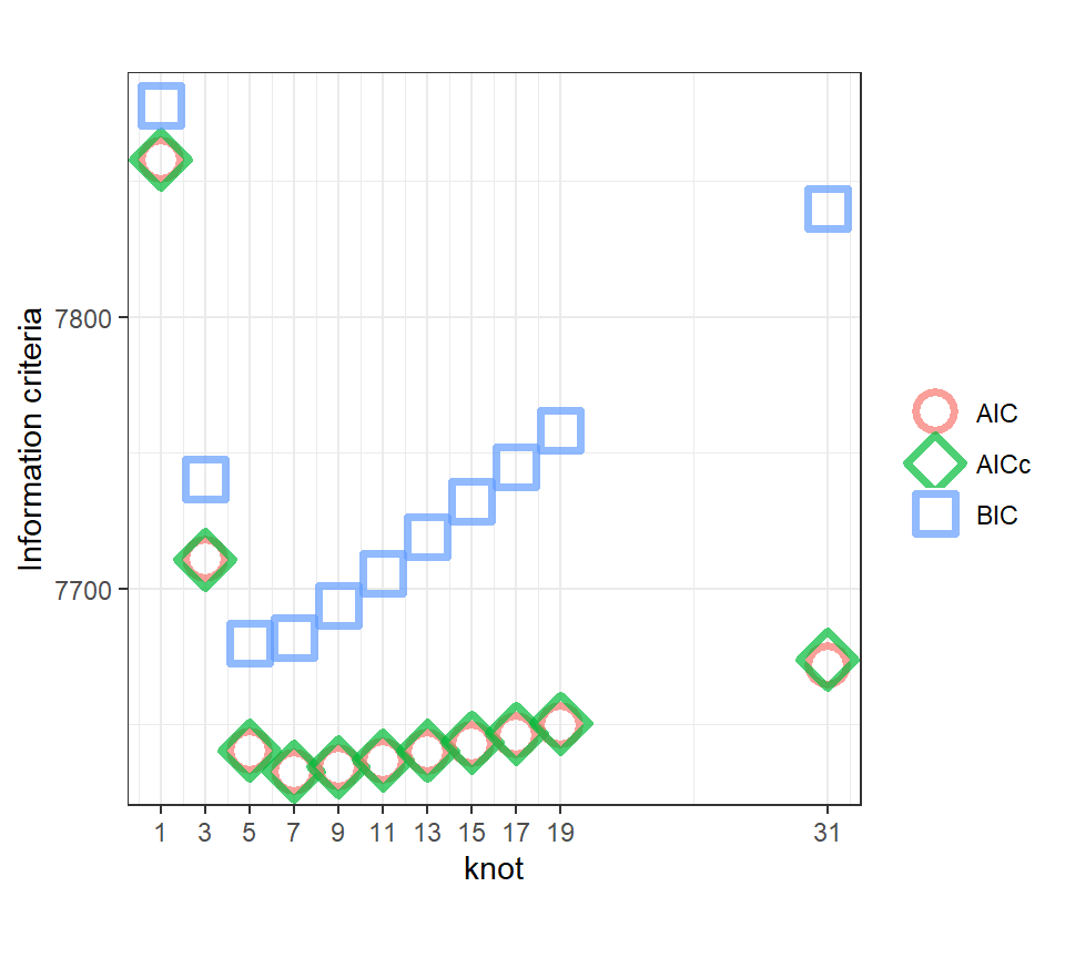
図3.10: AIC, AICc, BIC of the models with different number of knots.
しかし、毎回このように様々なノット数でモデリングを行い、情報量規準などに基づいた比較を行うのは時間がかかってしまう。そこで考えられたのが次節(3.8)で説明するpenalized spline modelと呼ばれるものである。
3.8 Penalized quadratic spline regression
各モデルにおいて、回帰係数などのパラメータは最小二乗法によって推定されている。すなわち、以下で表される残差平方和が最小になるように推定を行っている。
\[ Minimize\; over \;\mathbf{\beta} : \sum_i \epsilon_i^2 \]
行列形式で表すと以下のようになる。
\[
Minimize\; over \;\mathbf{\beta} : ||\mathbf{\epsilon^2}|| = ||\mathbf{Y} - \mathbf{X} \times \mathbf{\beta}||^2
\]
このとき、\(\mathbf{\beta}\)の推定値は以下の通りである(第1章も参照)。
\[ \hat{\mathbf{\beta}} = (\mathbf{X^t} \times \mathbf{X})^{-1} \times \mathbf{X^t} \times y \]
さて、ここで式(3.2)に従う二次スプライン回帰モデルを考える。もし両端を除くノット数がKであるとき、\((Depth-k_j)_+^2\)の回帰係数${11}, {12}, , _{1K} $を推定することになる。これらのパラメータは平滑化曲線(回帰曲線)の形に柔軟性を与える(= 形を調整する)役割を担っている。
ノット数を変えることで曲線の形を調整することはできるが、図3.9で見たようにノット数によって曲線の形は大きくは変わらなかった。そこで、ノット数を変えるのではなく、ノット数は固定して推定されるパラメータに制限をかけることでsmootherの形を調整するアプローチを考える。例えば、パラメータ\(\beta_{11}, \beta_{12}, \dots, \beta_{1K}\)の二乗がある定数\(C\)以下になるように推定を行うことを考える。
\[ \beta_{11}^2 + \beta_{12}^2 + \cdots + \beta_{1K}^2 < C \tag{3.6} \]
こうした方法は制限付き最適化(constrained optimization)と呼ばれる。
ある条件内で残差平方和を最小化するパラメータはラグランジュの未定乗数法と呼ばれる方法で推定できる。例として、条件下で以下の関数\(f(x,y)\)を最大にする\(x,y\)の組み合わせを探すことを考える。
\[ \begin{aligned} f(x,y) = 2x^2 + 2y^2 \:\: subject \:\: to \:\: x + y = 1 \end{aligned} \]
まず、以下の関数\(f(x,y,\lambda)\)を考える。
\[
f(x,y,\lambda) = 2x^2 + 2y^2 + \lambda(x + y-1)
\]
次に、\(f(x,y,\lambda)\)をそれぞれの変数について偏微分した値が全て0になるように連立方程式を解く。
\[
\begin{aligned}
4x + \lambda &= 0\\
4y + \lambda &= 0\\
x + y -1 &= 0
\end{aligned}
\]
すると、簡単に\(x = 1/2, y= 1/2\)と解けるが、これが条件の下で\(f(x,y)\)を最大化する\(x\)と\(y\)の値である。制限付き最適化についてもまったく同じことを行う。式(3.6)のような条件があるときに\(||\mathbf{Y} - \mathbf{X} \times \mathbf{\beta}||\)を最小化するパラメータを求めるには、以下を最小化すればよい。
\[ ||\mathbf{Y} - \mathbf{X} \times \mathbf{\beta}|| + \lambda \times (\beta_{11}^2 + \beta_{12}^2 + \cdots + \beta_{1K}^2 + C) \tag{3.7} \]
以下のような\(K+3\)次元の行列(\(K\)はノット数)\(\mathbf{D}\)とベクトル\(\mathbf{\beta}\)を定義する。
\[
\mathbf{D} =
\begin{bmatrix}
0 & \cdots & \quad & \quad & \cdots& 0\\
\vdots & 0 & \quad & \quad & \quad & \vdots\\
\quad & \quad & 0 & \quad & \quad & \quad \\
\quad & \quad & \quad & 1 \quad & \quad & \vdots\\
\vdots & \quad & \quad & \quad & \ddots & 0\\
0 & \cdots & \quad & \cdots & 0 & 1
\end{bmatrix}, \quad
\mathbf{\beta} = \begin{bmatrix}
\beta_1 \\
\beta_2\\
\beta_3\\
\beta_{11}\\
\vdots\\
\beta_{19}
\end{bmatrix}
\]
このとき、式(3.7)は以下のように変形できる。
\[ ||\mathbf{Y} - \mathbf{X} \times \mathbf{\beta}|| + \lambda \times (\mathbf{\beta^t} \times \mathbf{D} \times \mathbf{\beta} - \mathbf{C}) \tag{3.8} \]
これを\(\mathbf{\beta}\)について解くと、その推定値は以下のようになる。もし\(\lambda = 0\)ならば(= 何も条件がなければ)、推定値は通常の最小二乗法によるものと同じになる。
\[
\hat{\mathbf{\beta}} = (\mathbf{X^t} \times \mathbf{X} + \lambda \times \mathbf{D})^{-1} \times \mathbf{X^t} \times \mathbf{y} \tag{3.9}
\]
\(\lambda\)が特定の値を割り当てれば、smoother(\(f_{\lambda}\))を決定することができる。\(\hat{\beta}\)は\(\lambda\)の値によって変わるので、\(f_{\lambda}\)も\(\lambda\)によって変わる。\(\lambda\)はペナルティの大きさを表すので、大きいほどスプライン回帰を行わない通常の線形回帰や多項式回帰の結果に近づき、0ならば罰則のないスプライン回帰の結果と同じになる。
\[
\hat{f_{\lambda}} = \mathbf{X} \times \mathbf{\hat{\beta}} \tag{3.10}
\]
\(\lambda\)の値ごとの曲線を図示したのが図3.11である。\(\lambda\)が大きくなると2次の項までを含む普通の多項式回帰の結果に近づく。
K <- 9
D <- diag(rep(1, 3 + K))
D[1,1]<-D[2,2]<-D[3,3] <-0

X <- model.matrix(M3_5)
lambdas <- c(0, 0.25,0.7, 0.75, 1,10)
beta <- list()
Yhat <- list()

for (i in seq_along(lambdas)){
  beta[[i]] <- solve(t(X) %*% X + lambdas[i] * D) %*%t(X) %*% BL$Sources
  MyDepth <- seq(0.1, 1, length =100)
  XPred <- model.matrix(~ 1 + MyDepth + I(MyDepth^2)+
                        rhs2(MyDepth, q_Depth[1]) +
                        rhs2(MyDepth, q_Depth[2]) +
                        rhs2(MyDepth, q_Depth[3]) +
                        rhs2(MyDepth, q_Depth[4]) +
                        rhs2(MyDepth, q_Depth[5]) +
                        rhs2(MyDepth, q_Depth[6]) +
                        rhs2(MyDepth, q_Depth[7]) +
                        rhs2(MyDepth, q_Depth[8]) +
                        rhs2(MyDepth, q_Depth[9]))

  Yhat[[i]] <- XPred %*% as.vector(beta[[i]]) %>%
    data.frame() %>%
    rename(fitted = 1) %>%
    mutate(lambda = lambdas[i],
           Depth = MyDepth)
}

fitted_lambda <- bind_rows(Yhat[[1]], Yhat[[2]], Yhat[[3]], Yhat[[4]],
                           Yhat[[5]],Yhat[[6]]) %>%
  mutate(lambda_text = str_c("lambda = ", lambda))

BL %>%
  ggplot()+
  geom_point(aes(x = Depth, y = Sources),
             size = 2, alpha = 0.6, color = "grey54")+
  geom_line(data = fitted_lambda,
            aes(x = Depth, y = fitted),
            linewidth = 1)+
  facet_rep_wrap(~lambda_text, repeat.tick.labels = TRUE)+
  theme_bw(base_size = 12)+
  theme(aspect.ratio = 1,
        strip.background = element_blank(),
        strip.text = element_text(hjust = 0))+
  coord_cartesian(ylim = c(0,120), xlim = c(0.105,1))+
  labs(x = "Scaled depth", y = "Sources")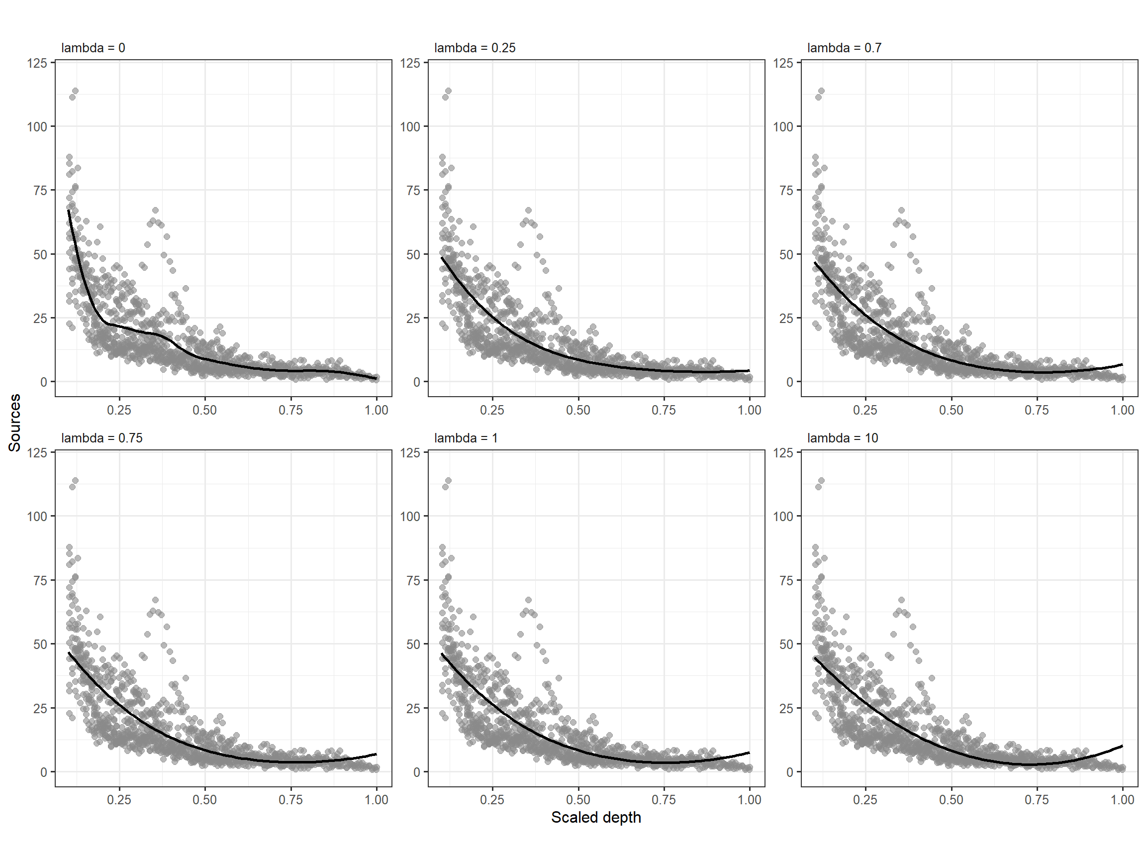
図3.11: Three smoothers using different values for λ
3.9 Other smoothers
mgcvパッケージやgamlssパッケージで用いられるsmootherには様々な種類がある。本節では、これらのいくつかについてまとめ、次節(3.10)では、3次平滑化スプラインについて詳しく解説する。
二次スプライン回帰(第3.5節)や罰則付きの二次スプライン回帰(第3.8節)では、以下の変数が説明変数(基底)となる。
\[ 1, Depth_i^2, (Depth_i - k_1)_+^2, (Depth_i - k_2)_+^2, \dots, (Depth_i - k_9)_+^2 \]
これは\(p\)次までの項を含むモデルについて以下のように一般化できる。このようなモデルはp次スプライン回帰モデルまたは罰則付きp次スプライン回帰と呼ばれる。
\[
1, Depth_i^2, (Depth_i - k_1)_+^p, (Depth_i - k_2)_+^p, \dots, (Depth_i - k_K)_+^p
\]
これらのモデルの問題点は各変数が強く相関している可能性が高いことである(特にノット数が多いときは)。Bスプライン平滑化(B-spline smoothing)と呼ばれる手法は、変数変換を施すことでこの問題を解決する。
絶対値の\(p\)乗項を含むモデルを考えることもできる。そのようなsmootherは放射基底平滑化(radial basis smoother)と呼ばれ、以下の基底を含む。
\[ 1, Depth_i^2, |Depth_i - k_1|^p, |Depth_i - k_2|^p, \dots, |Depth_i - k_K|^p \]
3.10 Cubic smoothing spline
第3.8節でやったように\(\beta_{11}, \dots, \beta_{1K}\)に制限を設けるのではなく、smootherの二次導関数(二回微分値)の和に制限を設ける方法もある。その場合、以下を最小化するようなパラメータを推定する。このような方法を平滑化スプライン(smoothing spline)という。
\[ ||\mathbf{Y} - \mathbf{X} \times \mathbf{\beta}||^2 + \lambda \times 全ポイントでの二次導関数の和 \tag{3.11} \]
一般にsmoother(\(f(x)\))の二次導関数を\(f''(x)\)とするとき、\(f''(x)\)の値が低いほど\(f(x)\)はより直線的であることを示す。全ての\(x\)について\(f''(x)\)の値を合計するためには、\(f''(x)\)を積分してやればよい。
そのため、式(3.11)は以下のように書き直せる。
\[
||\mathbf{Y} - \mathbf{X} \times \mathbf{\beta}||^2 + \lambda \times \int f''(x) dx \tag{3.12}
\]
Wood (2017) は、この基準で最小になる\(f(x)\)が3次スプラインであることを証明している。また、式(3.12)は式(3.8)のように書き直すことが分かっているので、\(\beta\)の推定値を得るのに積分をする必要はなく、式(3.9)で求めることができる。
\(\mathbf{\beta}\)を推定するためには、\(\mathbf{X}\)とパラメータ\(\lambda\)、罰則を表す行列\(\mathbf{D}\)を知る必要がある。3次平滑化スプライン(cubic smoothing spline)の基本は3次回帰スプライン(cubic regression spline)と同じなので、\(\mathbf{X}\)は同じものを用いることができる。
両端を除くノット数はこれまでと同様に9とする。
\(\mathbf{D}\)は\(11\times 11\)の正方行列で、成分は第3.6で出てきた\(R(X,z)\)によって決まる。\(\mathbf{D}(i + 2, j + 2)\)は\(R(x_i,x_j)\)によって決まり、\(x_iとx_j\)は両端を除くノットの値である。
Rでは以下の関数で計算できる。
spl.S <- function(xk){
  q <- length(xk) + 2
  S <- matrix(0, nrow = q, ncol = q)
  S[3:q, 3:q] <- outer(xk, xk, FUN = rk)
  S
}

D <- spl.S(q_Depth)最後に、\(\lambda\)については交差検証(第2.4節を参照)を行うことで最適な値を決定する。例えば、\(\lambda\)を0から0.01の間に25個とるとき、交差検証スコアは以下のように算出できる。
K <- 25
OCV <- vector(length = K)
lambda <- seq(0,0.001, length.out = K)
N <- nrow(BL)

for(j in 1:K){
  lambdas <- lambda[j]
  EP <- vector(length = N)
  for(i in 1:N){
    # i番目のデータを除く
    Xi <- X[-i, ]
    betai <- solve(t(Xi) %*% Xi + lambdas * D) %*%t(Xi) %*% BL$Sources[-i]
    Yi <- X[i,] %*% betai
    EP[i] <- BL$Sources[i] - Yi
  }
  OCV[j] <- sum(EP^2)/N
}図示すると以下のようになり、\(\lambda = 0.000208\)のときに交差検証スコアが最も低くなることが分かる(図3.12)。
data.frame(lambda = lambda,
           OCV = OCV) %>%
  arrange(OCV) -> ocv

ocv %>%
  ggplot(aes(x = lambda, y = OCV))+
  geom_line()+
  geom_point(x= ocv[1,1], y = ocv[1,2],
             color = "red2", size = 5)+
  annotate(geom = "text",
          x= ocv[1,1]+ 0.000002, y = ocv[1,2] + 0.05,
          label = str_c("lambda = ", round(ocv[1,1],5)))+
  geom_segment(x= ocv[1,1] + 0.00002, y = ocv[1,2] + 0.04,
               xend = ocv[1,1], yend = ocv[1,2])+
  theme_bw()+
  theme(aspect.ratio = 1)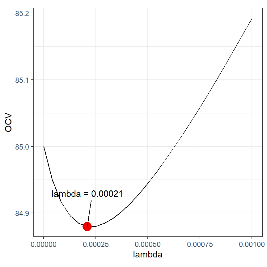
図3.12: OCV score plotted versus λ for the cubic smoothing spline.
データが多いときには上記の交差検証スコアを算出するのは非常に時間がかかるが、交差検証スコアは以下の式で計算できることが数学的にわかっている。なお、\(A_{ii}\)はハット行列\(\mathbf{S}\)の対角成分である(後述)。
\[ V_0 = \frac{1}{n}\sum_{i = 1} ^n (Y_i - \hat{f(X_i)})^2/(1-A_{ii}) \]
こちらの交差検証スコアは以下のように計算できる。
OCV2 <- vector(length = K)

for(i in 1:K){
    lambdas <- lambda[i]
    S <- X%*%solve(t(X) %*% X + lambdas * D) %*%t(X)
    Sii <- diag(S)
    fit <- S %*% BL$Sources
    E <- BL$Sources - fit
    OCV2[i] <- (1/N) *sum((E/(1-Sii))^2)
}
これは先ほど計算した交差検証スコアと全く同じ値を与える。
さて、ここまでの説明で\(\mathbf{X}\)、\(\mathbf{D}\)、\(\lambda\)を求めることができたので、\(\mathbf{\beta}\)を求めてsmootherを描くことができる。
## 先敵のlambda
lambda_opt <- ocv[1,1]

## betaの推定値
beta <- solve(t(X) %*% X + lambda_opt*D) %*% t(X) %*% BL$Sources

## 図示用の行列X
nd <- data.frame(Depth = seq(min(BL$Depth), max(BL$Depth), length = 100))
Xp <- spl.X(nd$Depth, q_Depth)

## smoother
fitted_css <- data.frame(fit = Xp%*%beta) %>%
bind_cols(nd)図3.13は推定された回帰曲線を図示したものである。
BL %>%
  ggplot()+
  geom_point(aes(x = Depth, y = Sources),
             size = 2, alpha = 0.6, color = "grey54")+
  geom_line(data = fitted_css,
            aes(x = Depth, y = fit),
            linewidth = 1)+
  theme_bw(base_size = 12)+
  theme(aspect.ratio = 1,
        strip.background = element_blank(),
        strip.text = element_text(hjust = 0))+
  coord_cartesian(ylim = c(0,120), xlim = c(0.105,1))+
  labs(x = "Scaled depth", y = "Sources")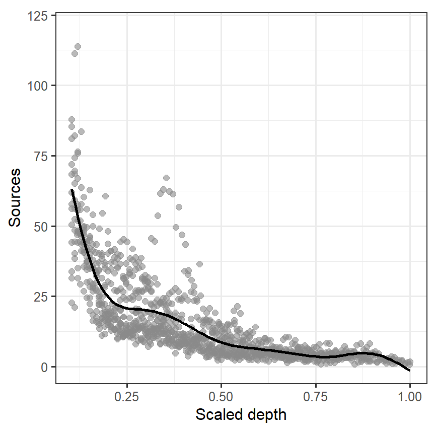
図3.13: Estimated cubic smoothing spline for the bioluminescence data.
3.11 Summary of smoother types
これまで見てきた手法では、以下の4つの手法でsmootherの形を調整してきた。
- 移動平均や局所回帰の範囲を変更する。
- スプライン回帰のノット数を変更する(= linear or quadratic spline regression)。
- パラメータに対して制限を設ける(= 制限付き最適化)
- 二次導関数に対して制限を設ける(= cubic smoothing spline)
3.12 Degree of freedom of smoother
式(3.9)回帰係数のパラメータ\(\mathbf{\beta}\)は以下の式で与えられる。
\[ \hat{\mathbf{\beta}} = (\mathbf{X^t} \times \mathbf{X} + \lambda \times \mathbf{D})^{-1} \times \mathbf{X^t} \times \mathbf{y} \]
また、式(3.10)で見たようにsmootherは以下のように書ける。
\[
\hat{f(_{\lambda})} = \mathbf{X} \times \hat{\mathbf{\beta}}
\]
これらを合わせると、以下のように書ける。
\[
\begin{aligned}
\hat{y} &= \hat{f_{\lambda}} = \mathbf{X} \times (\mathbf{X^t} \times \mathbf{X} + \mathbf{\lambda} \times \mathbf{D})^{-1} \times \mathbf{X^t} \times \mathbf{y} \\
&= S_{\mathbf{\lambda}} \times \mathbf{y}
\end{aligned}
\]
ここで、\(\mathbf{S_{\lambda}}\)は重回帰分析のときに出たハット行列(第1章参照)と同じ役割を持っている。第1章で、重回帰分析については自由度はハット行列の対角成分を合計することで得られることを見た。smootherの自由度も\(\mathbf{S_{\lambda}}\)の対角成分の合計によって求めることができる。
X <- spl.X(BL$Depth, q_Depth)
D <- spl.S(q_Depth)
lambda_opt <- ocv[1,1]

## Sを求める
S.lambda <- X %*% solve(t(X)%*%X + lambda_opt*D) %*%t(X)

## 自由度を求める
df1 <- sum(diag(S.lambda))

df1
## [1] 10.1985よって、smootherの自由度は10.1985018である。なお、\(\lambda\)の値が大きいほど自由度は小さくなる。\(\lambda\)の値によって自由度がどう変わるかをプロットしたのが図3.14)だが、このことが確かめられる。
df <- vector()
lambda <- seq(0,5,length = 200)

for(i in seq_along(lambda)){
  S.lambda <- X %*% solve(t(X)%*%X + lambda[i]*D) %*%t(X)
  df[i] <- sum(diag(S.lambda))
}

data.frame(lambda = lambda,
           df = df) %>%
  ggplot(aes(x = lambda, y = df))+
  geom_line()+
  theme_bw()+
  theme(aspect.ratio = 1)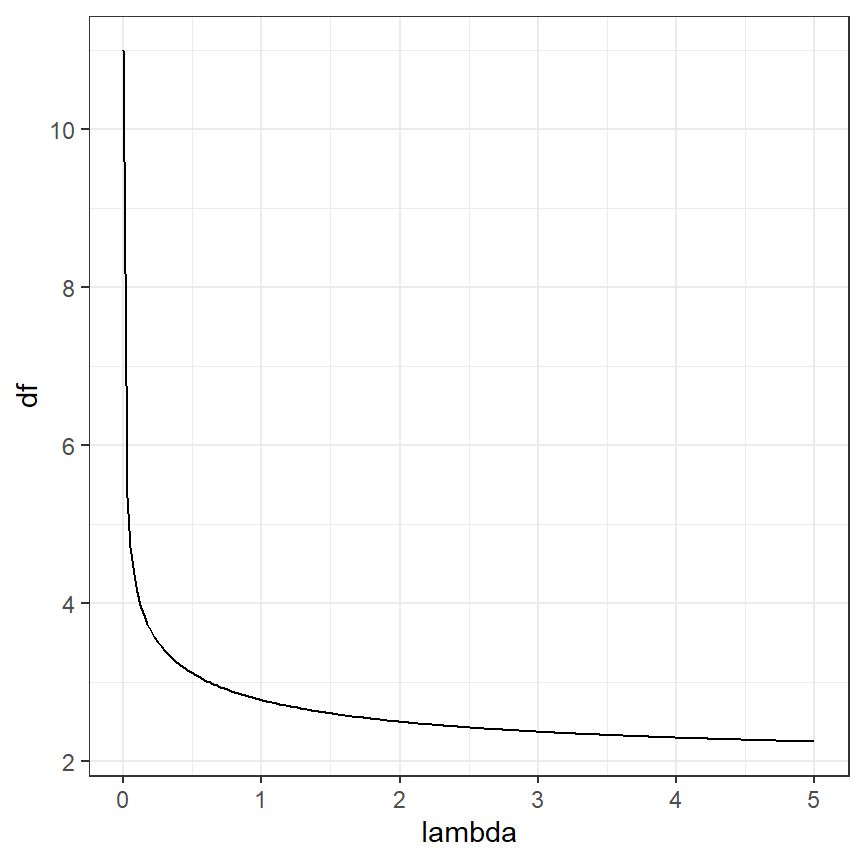
図3.14: Effective degrees of freedom plotted versus λ.
3.13 Bias-variance trade-off
続いて、smootherの信頼区間を計算することを考える。その前に、“bias-variance trade off”について学ぶ必要がある。
あるsmootherについての平均二乗誤差(mean squared error: MSE)は以下のように定義できる。なお、\(f(Depth_i)\)は真のsmootherである。
\[ MSE(\hat{f_{\lambda}}(Depth_i)) = E \Bigl( \bigl( \hat{f_{\lambda}}(Depth_i) - f(Depth_i) \bigl)^2 \Bigl) \]
これは、以下のように変形することができる。式の前半部分はバイアス(推定されたsmootherと真のsmootherの差)を表し、後半部分は推定されたsmootherの分散を表す。\(\lambda\)が小さいとき、推定されたsmootherはより非線形性が強いのでバイアスは小さくなるが、推定されたsmoother内でのばらつきは大きくなる。\(\lambda\)が大きいときはこの逆である。すなわち、バイアスと分散の間にはトレードオフの関係がある。
\[ MSE(\hat{f_{\lambda}}(Depth_i)) = \Bigl(E \bigl( \hat{f_{\lambda}}(Depth_i) \bigl)- f(Depth_i) \Bigl) ^2 + var \bigl(\hat{f_{\lambda}}(Depth_i)\bigl) \]
3.14 Confidence intervals
今回取り上げたsmootherについて、モデルから推定される高原の数の推定値(\(\hat{\mathbf{y}}\))とその分散共分散行列は以下のように書ける。標準偏差は分散共分散行列の対角成分の1/2乗であり、信頼区間はそれの-2倍と2倍した区間となる(正確には自由度を考慮する必要がある)。
\[ \begin{aligned} \hat{\mathbf{y}} &= \hat{f} = \mathbf{S_{\lambda}} \times \mathbf{y}\\ cov(\hat{f}) &= \sigma^2 \times \mathbf{S_{\lambda}} \times \mathbf{S_{\lambda}}^t \end{aligned} \]
分散\(\sigma^2\)を求めるためには、error degrees of freedomを求める必要がある。これは、以下の式で求められる。なお、\(tr()\)は行列の対角成分の和を計算する関数である。
\[ N - tr(2 \times \mathbf{S_{\lambda}} - \mathbf{S_{\lambda}} \times \mathbf{S_{\lambda}}^t) \]
分散の推定値は以下の式で求められる。なお、\(df_{error}\)はerror degrees of freedomである。
\[ (\mathbf{y} - \mathbf{X} \times \hat{\beta})^2/df_{error} \]
Rでは以下のように求められる。
## error degrees of freedom
df.Error <- nrow(BL) - sum(diag(2*S.lambda - S.lambda %*% t(S.lambda)))

## sigma
sigma2 <- sum((BL$Sources - X%*%beta)^2)/df.Error
(sigma <- sqrt(sigma2))
## [1] 9.11692さて、それでは\(\sigma\)が求まったのが標準誤差を計算することができる。図3.13で回帰曲線を描いたときに使用した行列\(X_p\)について標準誤差を算出すると以下のようになる。se_predYがそれぞれの\(Depth\)の値のときの標準誤差である。
Sp.lambda <- Xp %*% solve(t(Xp)%*%Xp + lambda_opt*D) %*%t(Xp)
cov_predY <- sigma2 * Sp.lambda %*% t(Sp.lambda)
se_predY <- sqrt(diag(cov_predY))よって、95%信頼区間付きの回帰曲線は以下のように書ける(図3.15)。
fitted_css %>%
  mutate(lower = fit - se_predY*qt(0.975, df = df1),
         upper = fit + se_predY*qt(0.975, df = df1)) -> fitted_css2

BL %>%
  ggplot()+
  geom_point(aes(x = Depth, y = Sources),
             size = 2, alpha = 0.2, color = "grey54")+
  geom_line(data = fitted_css2,
            aes(x = Depth, y = fit),
            linewidth = 1)+
  geom_ribbon(data = fitted_css2,
            aes(x = Depth, y = fit, ymin = lower, ymax = upper),
            color = "black", alpha = 0, linetype = "dashed",
            linewidth = 1)+
  theme_bw(base_size = 12)+
  theme(aspect.ratio = 1,
        strip.background = element_blank(),
        strip.text = element_text(hjust = 0))+
  coord_cartesian(ylim = c(0,120), xlim = c(0.105,1))+
  labs(x = "Scaled depth", y = "Sources")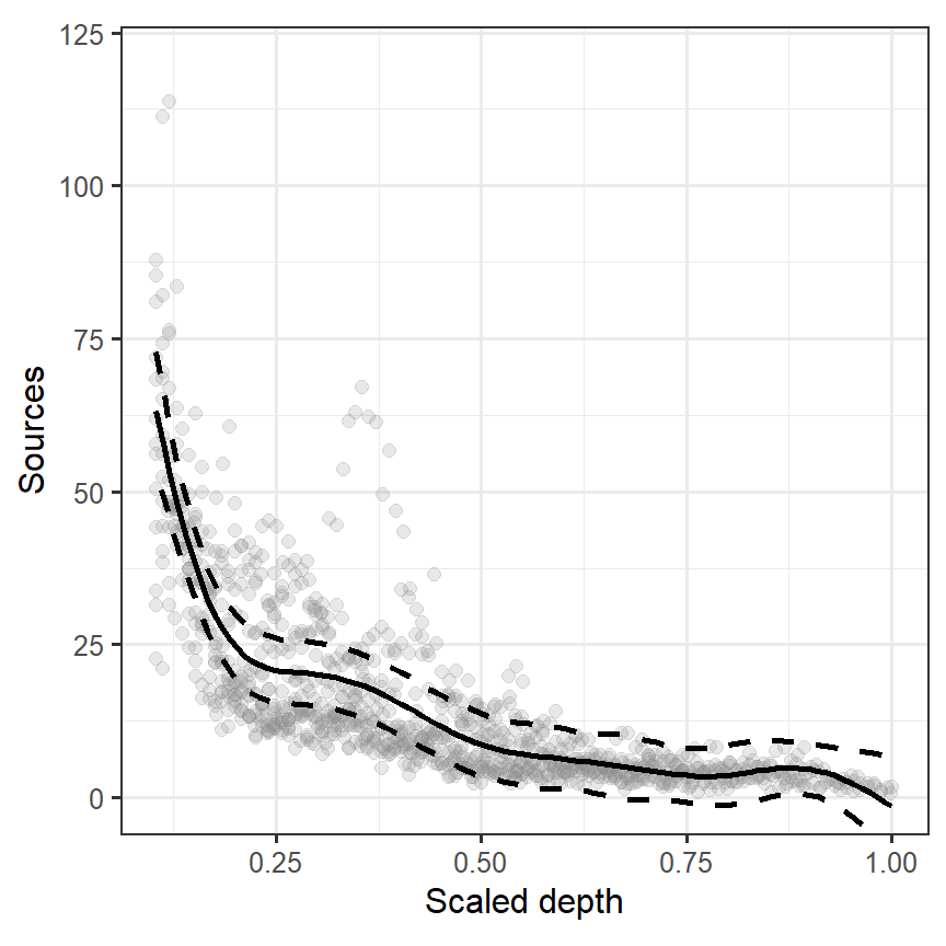
図3.15: Estimated cubic smoothing spline for the bioluminescence data with 95% confidence interval.
しかし、こうして求めた信頼区間には問題がある。求めた信頼区間は、推定されたsmoother(yfit = Xp %*% beta)がバイアスのない推定値だと仮定したうえで計算されたものである。もしsmootherの推定値にバイアスがあるのであれば、図3.15で図示した区間を信頼区間とはみなせない。
mgcvパッケージでは、バイアスに対処するために補正を行っている。
3.15 Using the function gam in mgcv
mgcvパッケージを用いたGAMは以下のように実行できる。gam関数は前節までの方法と似ているが、より洗練された方法を用いてsmootherの推定を行っている。
推定結果は以下の通り。smootherの自由度は8.496で推定された切片は16.7455である。GCV scoreは、一般化交差検証のスコアである。
##
## Family: gaussian
## Link function: identity
##
## Formula:
## Sources ~ s(Depth)
##
## Parametric coefficients:
##             Estimate Std. Error t value Pr(>|t|)
## (Intercept)  16.7455     0.2847   58.83   <2e-16 ***
## ---
## Signif. codes:  0 '***' 0.001 '**' 0.01 '*' 0.05 '.' 0.1 ' ' 1
##
## Approximate significance of smooth terms:
##            edf Ref.df   F p-value
## s(Depth) 8.496  8.921 251  <2e-16 ***
## ---
## Signif. codes:  0 '***' 0.001 '**' 0.01 '*' 0.05 '.' 0.1 ' ' 1
##
## R-sq.(adj) =  0.681   Deviance explained = 68.4%
## GCV = 85.778 Scale est. = 85.001 n = 1049推定された回帰曲線(smoother)は以下のとおりである(図3.16)。
pred_M3_7 <- fitted_values(M3_7, data = nd)

## 描画
pred_M3_7 %>%
  ggplot(aes(x = Depth, y = fitted))+
  geom_line()+
  geom_ribbon(aes(ymin = lower, ymax = upper),
              color = "black", alpha = 0, linetype = "dashed",
            linewidth = 1) +
  geom_point(data = BL,
             aes(y = Sources),
             size = 2, alpha = 0.2, color = "grey54")+
  theme_bw(base_size = 12)+
  theme(aspect.ratio = 1,
        strip.background = element_blank(),
        strip.text = element_text(hjust = 0))+
  coord_cartesian(ylim = c(0,120), xlim = c(0.105,1))+
  labs(x = "Scaled depth", y = "Sources")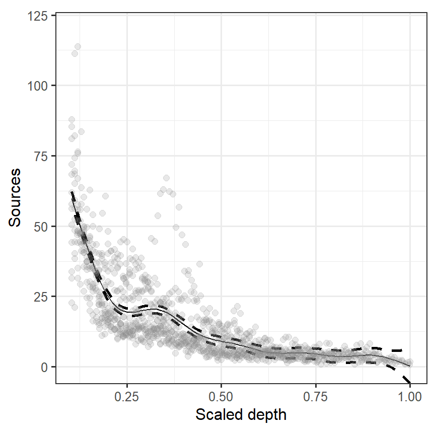
図3.16: Estimated smoother obtained by the gam function from the package mgcv for the bioluminescence data.
それでは、gam関数では実際にどのような手順で推定が行われているのだろうか。まず、s(Depth)としたときに何が行われているのだろうか。関数s()の引数はいくつかあるが、そのうちデフォルトで与えられているのは以下の3つである。
k = -1, fx = FALSE, bs = "tp"
fx = FALSEは、罰則付きの回帰スプラインが使われていることを表し、もしfx = TRUEならば自由度を固定した回帰スプラインが行われる。kはsmootherの基底の次元を表し、\(k-1\)がsmootherの自由度の上限になる。k = -1ではデフォルトの値が選ばれる。bsは使用されるsmootherが指定される。詳しい説明は?smoother.termsとすれば見ることができる。
つまり、引数を何も指定しないときは罰則付きの回帰スプラインが適用され、自由度は交差検証によって決定される。自由度を固定してGAMを実行するときは以下のようにすればよい。k = 5にするとsmootherの自由度は4になる。
使われるsmootherの種類による推定結果の違いは小さいが、データ数によっては種類を変えることで推定が効率的になったりする。デフォルトのbs = "tp"では薄板平滑化スプライン(thin plate regression spline)と呼ばれる方法が用いられる。この方法では交互作用項を含めた平滑化を行うことができるようだ(詳しくはこちらやこちら)。
bs = "cr"では、罰則付きの3次スプライン回帰が適用され、bs = "cc"では説明変数の両端のポイントが接続される場合(例えば月データの分析)に使える3次スプライン回帰である。
さて、最初のモデル(M3_7)の説明に戻ろう。モデルの予測値はfitted()関数で求めることができる。
##  [1] 59.75170 56.23345 52.72462 49.93488 46.49023 43.12257 39.86806 36.76435
##  [9] 34.41493 31.67422
パラメータ(回帰係数)の推定値は以下のように求められる。
## (Intercept)  s(Depth).1  s(Depth).2  s(Depth).3  s(Depth).4  s(Depth).5
##    16.74551   -46.31747   -56.49162   -34.94561   -43.55188   -38.29367
##  s(Depth).6  s(Depth).7  s(Depth).8  s(Depth).9
## 38.83802 -31.02217 -83.19786 -55.07702predict()関数でtype = "lpmatrix"とすると、モデルの説明変数を含む行列を得ることができる。
よって、モデルの予測値は以下のように求めることができる。
また、予測値の分散共分散行列は\(\mathbf{X} \times cov(\mathbf{\beta}) \times \mathbf{X^t}\)で求めることができるので(第1章参照)、以下のように求められる、
3.16 The danger of using GAM
これまで様々な方法でsmootherを推定してきたが、その多くではスケール化された水深が0.3から0.4のあたりで光源の数がわずかに増加していると推定された。しかし、これまではサンプリングを行ったステーションの影響は無視して分析を行ってきた(第3.1節も参照)。推定されたsmotherのパターンがこうした影響を受けていることはないだろうか。
まず、モデルの診断を行う。図3.17はモデルの予測値と残差の関係をプロットしたものである。明確なパターンがあり、等分散性の仮定が満たされていないことが分かる。
data.frame(fit = fitted(M3_7),
           resid = resid(M3_7)) %>%
  ggplot(aes(x = fit, y = resid))+
  geom_point()+
  geom_hline(yintercept = 0,
             linetype = "dotted")+
  theme_bw()+
  theme(aspect.ratio = 1)+
  labs(y = "Residuals", x = "Fitted values")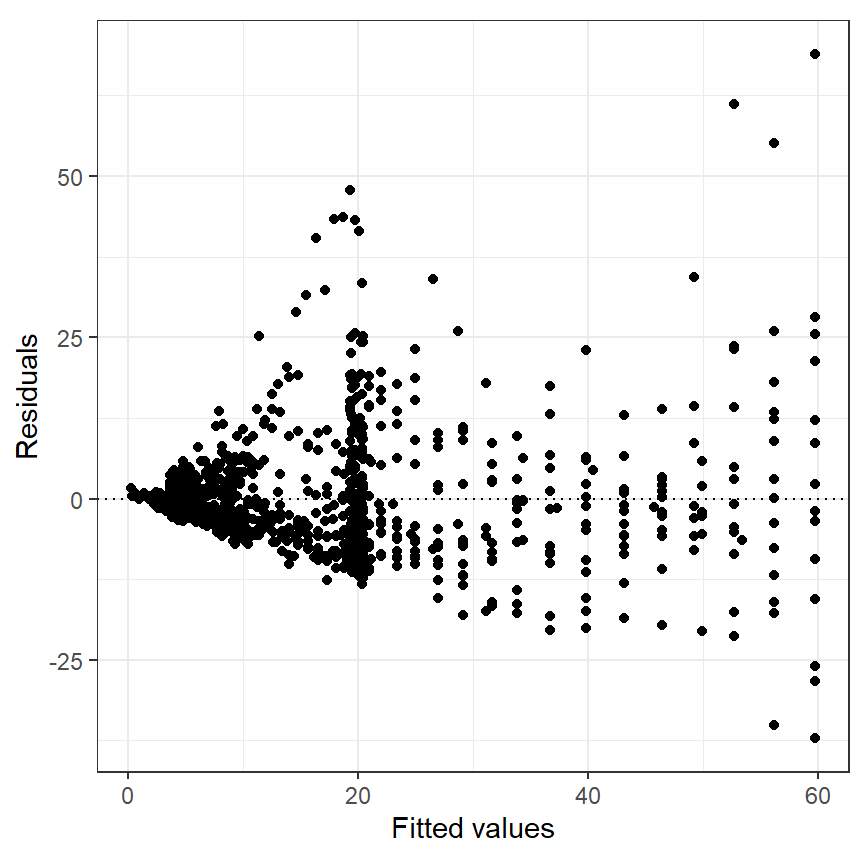
図3.17: Residuals plotted versus fitted values for the GAM using only depth as smoother.
図3.18は、ステーションごとの残差をプロットしたものである。ステーションごとにパターン(0以上が多い/0以下が多いなど)があることが分かる。
data.frame(resid = resid(M3_7),
           Station = as.factor(BL$Station)) %>%
  ggplot(aes(x = Station, y = resid))+
  geom_boxplot()+
  geom_hline(yintercept = 0,
             linetype = "dotted")+
  theme_bw()+
  theme(aspect.ratio = 1)+
  labs(y = "Residuals")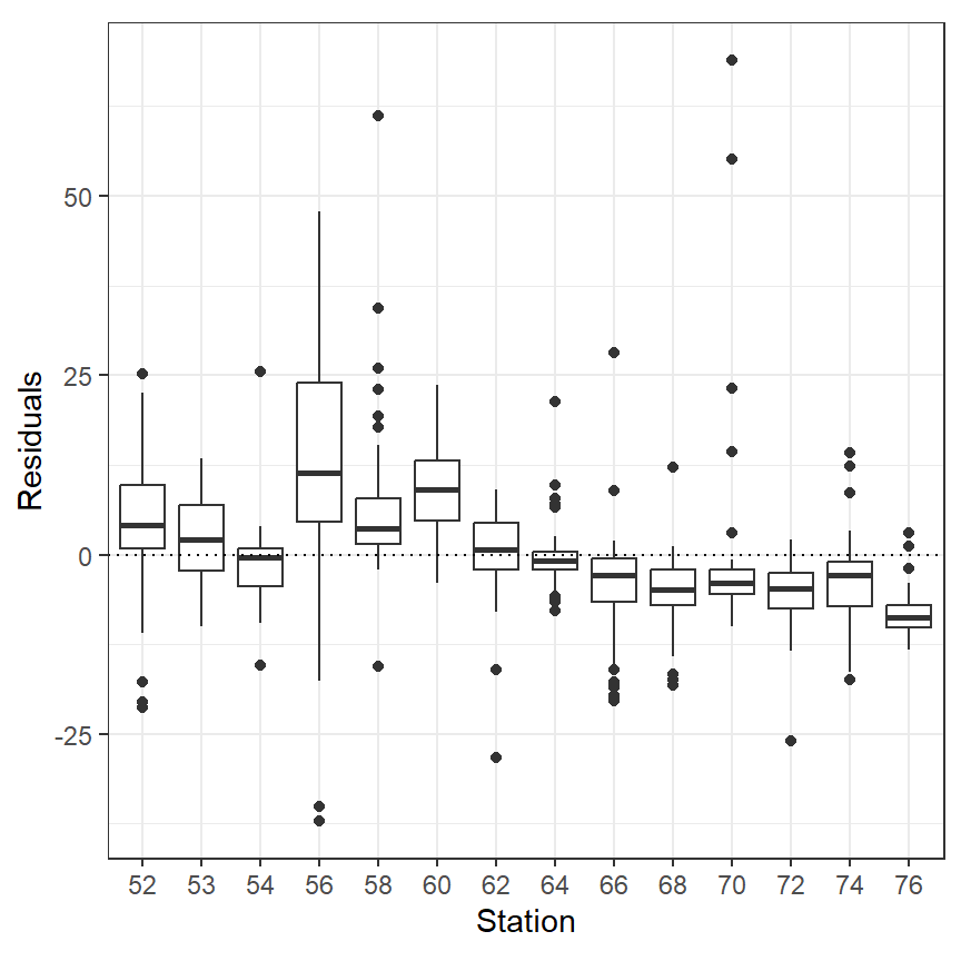
図3.18: Residuals plotted versus station for the GAM using only depth as smoother.
また、水深と残差の関係をステーションごとにプロットすると(図3.19)、ステーションごとに違う傾向があることが分かる。以上より、smootherとして\(f(Depth_i)\)だけを考えることが適当ではないことが示唆された。
data.frame(resid = resid(M3_7),
           Station = BL$Station,
           Depth = BL$Depth) %>%
  ggplot(aes(x = Depth, y = resid))+
  geom_point(alpha = 0.5,
             shape = 1)+
  facet_rep_wrap(~Station, repeat.tick.labels = TRUE)+
  theme_bw()+
  theme(aspect.ratio = 1,
        strip.background = element_blank(),
        strip.text = element_text(hjust = 0))+
  labs(y = "Residuals")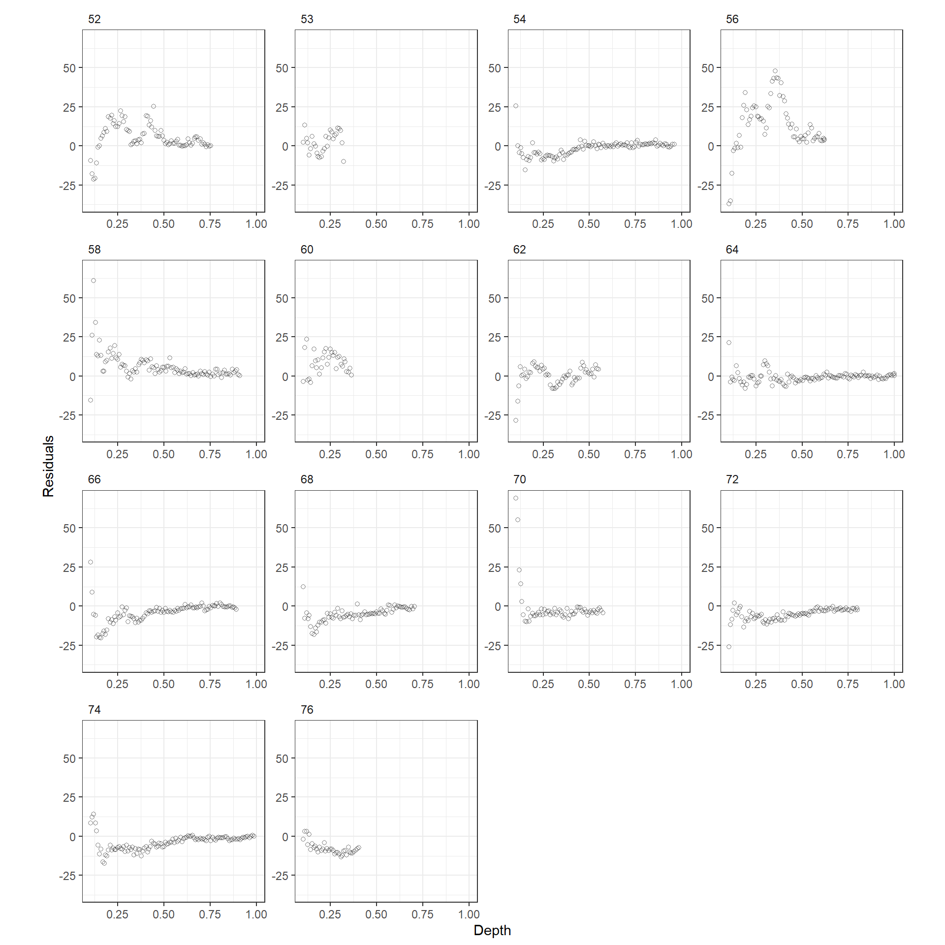
図3.19: Residuals plotted versus depth for each station for the GAM using only depth as smoother.
この問題を解決する方法としては、各ステーションに異なるsmootherを適用することなどがあるが、数が多すぎる。他の方法としては、渦巻き(Eddy)の有無によってsmootherを変えるというものである。
図3.20は、渦巻きの有無ごとに水深と光源の数の関係を描いた図である。明らかに渦巻きの有無ごとに傾きが異なっていることが分かる。
BL %>%
  mutate(Station = as.factor(Station)) %>%
  ggplot(aes(x = Depth, y = Sources))+
  geom_point(aes(color = Station))+
  facet_rep_wrap(~Eddy)+
  theme_bw()+
  theme(aspect.ratio = 1,
        strip.background = element_blank(),
        strip.text = element_text(hjust = 0))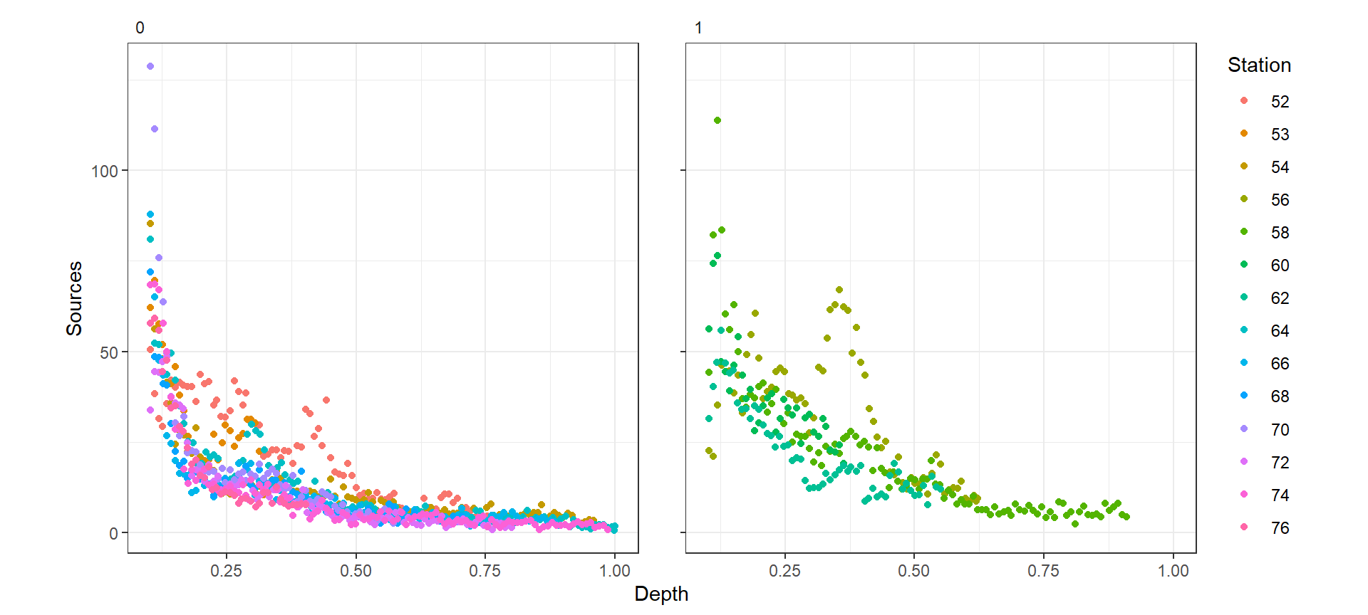
図3.20: Source s profiles plotted versus scaled depth for absence (left) and presence (right) of eddies. Each line corresponds to a station.
そこで、以下の渦巻きの有無ごとにsmootherが異なるモデルを考える。なお,\(j = 1,2\)で\(f_1(Depth_i)\)は渦巻きがないときのsmootherである。Stationは説明変数に入れた。
\[ \begin{aligned} Sources_i &= \alpha + f_j(Depth_i) + Station_i + \epsilon_i \\ \epsilon_i &\sim N(0,\sigma^2) \end{aligned} \]
Rでは、第2.6節で見たようにby =とすることで渦巻きの有無ごとのsmootherを推定できる。以下では、渦巻きの有無ごとにsmootherを推定する場合としない場合のモデルを作成する。
M3_8 <- gam(Sources ~ s(Depth) + factor(Station), data = BL)
M3_9 <-  gam(Sources ~ s(Depth, by = factor(Eddy)) + factor(Station), data = BL)
AICを比較すると、渦巻きの有無ごとにsmootherを推定したモデルの方がよいモデルであることが分かる。
推定された渦巻きの有無ごとのsmootherを図示したのが図3.21である。両者が異なるパターンを示していることが分かる。渦巻きがあり(Eddy = 1)のときに水深が深いところで95%信頼区間が狭くなっているのは、そのあたりのデータが少ないからである。
## M3_8
smooth_estimates(M3_9) %>%
  add_confint() %>%
  rename(Eddy = 7) %>%
  mutate(Eddy = str_c("Eddy = ", Eddy)) %>%
  ggplot(aes(x = Depth, y = est))+
  geom_line(aes(),
            linewidth = 1)+
  geom_ribbon(aes(ymin = lower_ci, ymax = upper_ci),
              alpha = 0,
              color = "black",
              linetype = "dashed",
              linewidth = 0.7)+
  facet_rep_wrap(~Eddy, repeat.tick.labels = TRUE)+
  theme_bw()+
  theme(aspect.ratio = 1,
        strip.background = element_blank(),
        strip.text = element_text(hjust = 0))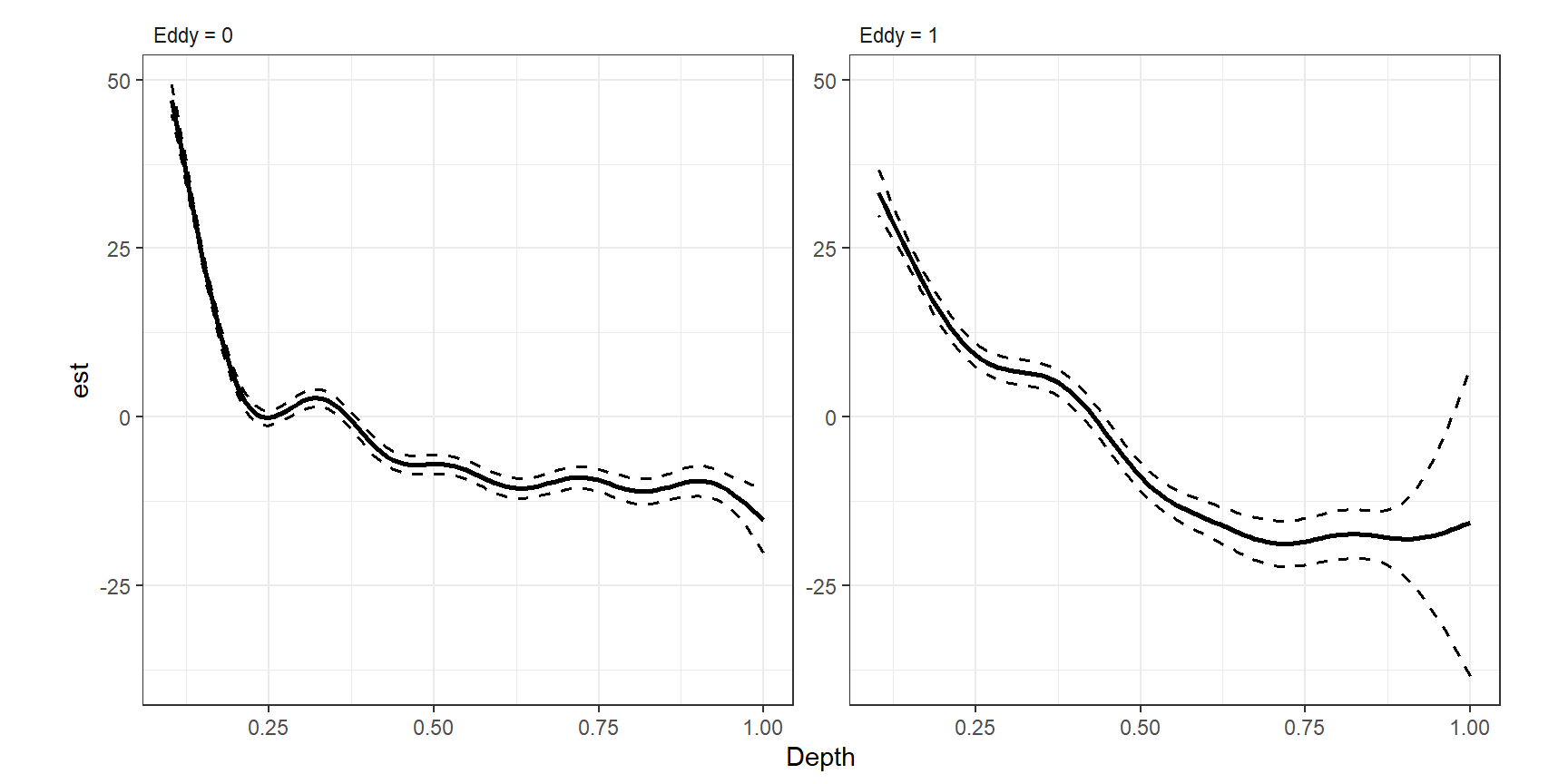
図3.21: Estimated smoothers for depth for absence (left) and presence (right) of eddies.
他の方法はランダム効果を用いる方法であるが、これについては別の本で解説を行っている(Zuur et al. 2014)。
3.17 Additive models with multiple smoothers
これまでのモデルは、一つの変数のsmootherのみを用いていた。これを二つ以上の変数のsmootherに拡張するのはシンプルである。
ここでは、蛍光物質(クロロフィル)の量(mg/L)(flcugl)のsmootherも加えたモデルを考える。
\[
\begin{aligned}
Sources_i &= \alpha + f_1(Depth_i) + f_2(flcugl_i) + Station_i + \epsilon_i \\
\epsilon_i &\sim N(0,\sigma^2)
\end{aligned}
\]
図3.22はDepthとflcugl、flcuglとSourcesの関係をプロットしたものである。flcuglには一つだけ外れ値があるので、以後の分析ではこれは除く。
BL %>%
  ggplot(aes(x = Depth, y = flcugl))+
  geom_point(shape = 1, alpha = 0.7)+
  theme_bw()+
  theme(aspect.ratio = 1) -> p1

BL %>%
  ggplot(aes(x =flcugl, y = Sources))+
  geom_point(shape = 1, alpha = 0.7)+
  theme_bw()+
  theme(aspect.ratio = 1) -> p2

p1 + p2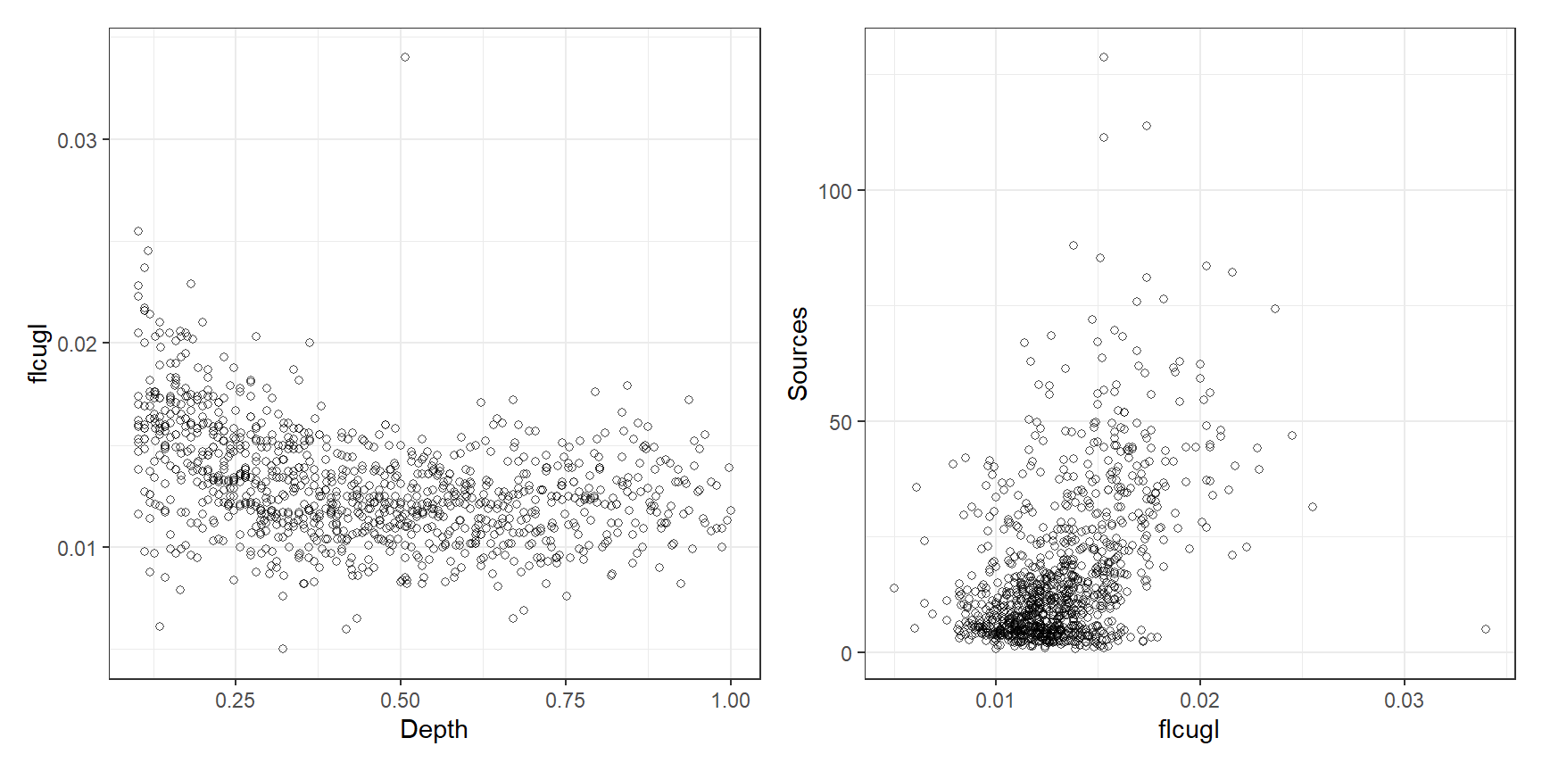
図3.22: Scatterplot of flcugl versus depth (left) and sources versus flcugl (right).
これまでと同様に、それぞれのsmootherは以下のように書ける。それぞれのsmootherについてノットの数と位置を決定する必要があるが、これは同じでも違くてもよい。また、それぞれのsmootherについて基底(\(b_{1j}(Depth_i),b_{2j}(flcugl_i)\))を決める必要がある。例えば、\(Depth\)については線形スプライン回帰を適用するが、\(flcugl\)については3次平滑化スプラインを適用する、ということもできる。
\[
\begin{aligned}
f_1(Depth_i) &= \sum_{j =1}^K \beta_{1j} \times b_{1j}(Depth_i)\\
f_2(flcugl_i) &= \sum_{j =1}^K \beta_{2j} \times b_{2j}(flcugl_i)\\
\end{aligned}
\]
モデル全体の切片\(\alpha\)があるので、各smootherの切片は除いて0の周りで周辺化する。各smootherのパラメータ\(\lambda_1, \lambda_2\)は交差検証によって決定され、自由度もそれに基づいて別々に計算される。
Rでは以下のように実行する。ここでは、両方のsmootherに3次平滑化スプラインを用いる。
BL2 <- BL %>% filter(flcugl < 0.03)

M3_10 <- gam(Sources ~ s(Depth, bs = "cr") + s(flcugl, bs = "cr") + factor(Station),
data = BL2)推定された各smootherは以下の通り(図3.23)。flcuglのsmootherはゆっくり増加したのち、急激に減少していることが分かる。Depthの方はほとんど変わらない。
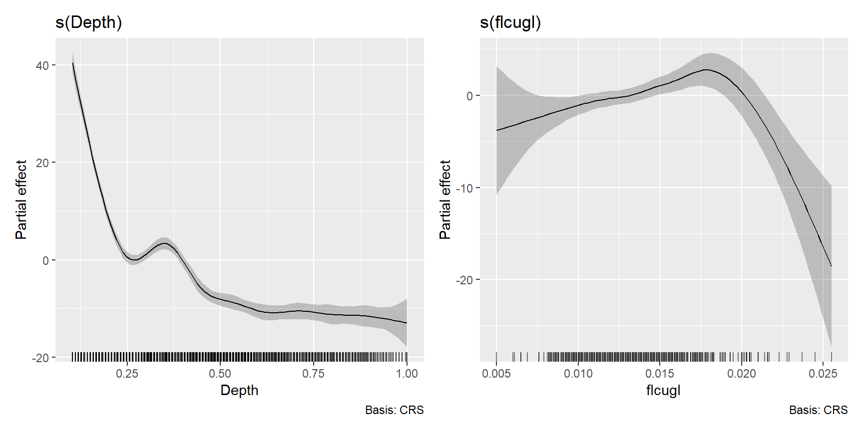
図3.23: Estimated cubic smoothing splines for Depth and fclugl.
モデルの要約は以下の通り。いずれのsmootherも有意であるが、このモデルでは渦巻きの有無の効果を無視している。flcuglの効果も渦巻きの有無によって異なるかもしれない。
##
## Family: gaussian
## Link function: identity
##
## Formula:
## Sources ~ s(Depth, bs = "cr") + s(flcugl, bs = "cr") + factor(Station)
##
## Parametric coefficients:
##                   Estimate Std. Error t value Pr(>|t|)
## (Intercept)        22.8401     0.8599  26.562  < 2e-16 ***
## factor(Station)53  -2.9374     1.6827  -1.746 0.081177 .
## factor(Station)54  -7.8883     1.1299  -6.981 5.27e-12 ***
## factor(Station)56   7.3880     1.3155   5.616 2.52e-08 ***
## factor(Station)58  -0.6668     1.1631  -0.573 0.566615
## factor(Station)60   2.8120     1.6417   1.713 0.087039 .
## factor(Station)62  -5.2367     1.3584  -3.855 0.000123 ***
## factor(Station)64  -7.1549     1.1269  -6.349 3.25e-10 ***
## factor(Station)66 -10.3260     1.1471  -9.002  < 2e-16 ***
## factor(Station)68 -11.1717     1.2177  -9.175  < 2e-16 ***
## factor(Station)70  -6.7784     1.2997  -5.216 2.22e-07 ***
## factor(Station)72 -11.4385     1.1723  -9.757  < 2e-16 ***
## factor(Station)74 -10.2104     1.1278  -9.053  < 2e-16 ***
## factor(Station)76 -13.6073     1.5054  -9.039  < 2e-16 ***
## ---
## Signif. codes:  0 '***' 0.001 '**' 0.01 '*' 0.05 '.' 0.1 ' ' 1
##
## Approximate significance of smooth terms:
##             edf Ref.df       F  p-value
## s(Depth)  8.567  8.937 214.603  < 2e-16 ***
## s(flcugl) 5.338  6.529   5.856 3.45e-06 ***
## ---
## Signif. codes:  0 '***' 0.001 '**' 0.01 '*' 0.05 '.' 0.1 ' ' 1
##
## R-sq.(adj) =  0.791   Deviance explained = 79.7%
## GCV = 57.163 Scale est. = 55.641 n = 1048そこで、以下の7つのモデルを作成してAICによるモデル比較を行う。交互作用を考慮する2次元のsmootherがあるモデル(M3_11_hとM3_11_i)については第6章で触れる。
## Depthのみ、Eddyによる違いなし
M3_11_a <- gam(Sources ~ s(Depth, bs = "cr") + factor(Station), data = BL2)

## flcuglのみ、Eddyによる違いなし
M3_11_b <- gam(Sources ~ s(flcugl, bs = "cr") + factor(Station), data = BL2)

## Depthとflcugl。DepthのみEddyによる違いあり
M3_11_c <- gam(Sources ~ s(Depth, bs = "cr", by = factor(Eddy)) +
                 s(flcugl, bs = "cr") + factor(Station), data = BL2)

## Depthとflcugl。flcuglのみEddyによる違いあり
M3_11_d <- gam(Sources ~ s(Depth, bs = "cr") +
                 s(flcugl, bs = "cr", by = factor(Eddy)) + factor(Station), data = BL2)

## Depthとflcugl、両方がEddyによって異なる
M3_11_e <- gam(Sources ~ s(Depth, bs = "cr", by = factor(Eddy)) +
                 s(flcugl, bs = "cr", by = factor(Eddy)) + factor(Station), data = BL2)

## DepthのみでEddyによって異なる。flcuglは普通の説明変数として入れる。
M3_11_f <- gam(Sources ~ s(Depth, bs = "cr", by = factor(Eddy)) + flcugl + factor(Station),
               data = BL2)

## DepthのみでEddyによって異なる。flcuglとEddyの交互作用を入れる。
M3_11_g <- gam(Sources ~ s(Depth, bs = "cr", by = factor(Eddy)) + flcugl*factor(Eddy) +
                 factor(Station), data = BL2)

## Depthとflcuglの交互作用を考える。Eddyによる傾きの違いなし。
M3_11_h <- gam(Sources ~ te(Depth, flcugl) + factor(Station), data = BL2)

## Depthとflcuglの交互作用を考える。Eddyによる傾きの違いあり。
M3_11_i <- gam(Sources ~ te(Depth, flcugl,  by = factor(Eddy))
+ factor(Station), data = BL2)モデル比較の結果、どちらのsmootherも渦巻きの有無によって異なるM3_11_eが最も良いよう。
AIC(M3_10, M3_11_a, M3_11_b,M3_11_c,M3_11_d,M3_11_e,M3_11_f,M3_11_g,M3_11_h,M3_11_i) %>%
  data.frame() %>%
arrange(AIC)M3_11_eのsmootherを図示すると以下のようになる(図3.24)。
smooth_estimates(M3_11_e) %>%
  add_confint() %>%
  pivot_longer(cols = c(Depth, flcugl)) %>%
  drop_na(value) %>%
  rename(Eddy = 6) %>%
  mutate(Eddy = str_c("Eddy = ", Eddy)) %>%
  ggplot(aes(x = value, y = est))+
  geom_line()+
  geom_ribbon(aes(ymin = lower_ci, ymax = upper_ci),
              alpha = 0, color = "grey29", linewidth = 0.9,
              linetype = "dashed")+
  labs(x = "x", y = "")+
  theme_bw()+
  theme(aspect.ratio = 1)+
  facet_rep_grid(Eddy~name, scales = "free_x",
                 repeat.tick.labels = TRUE)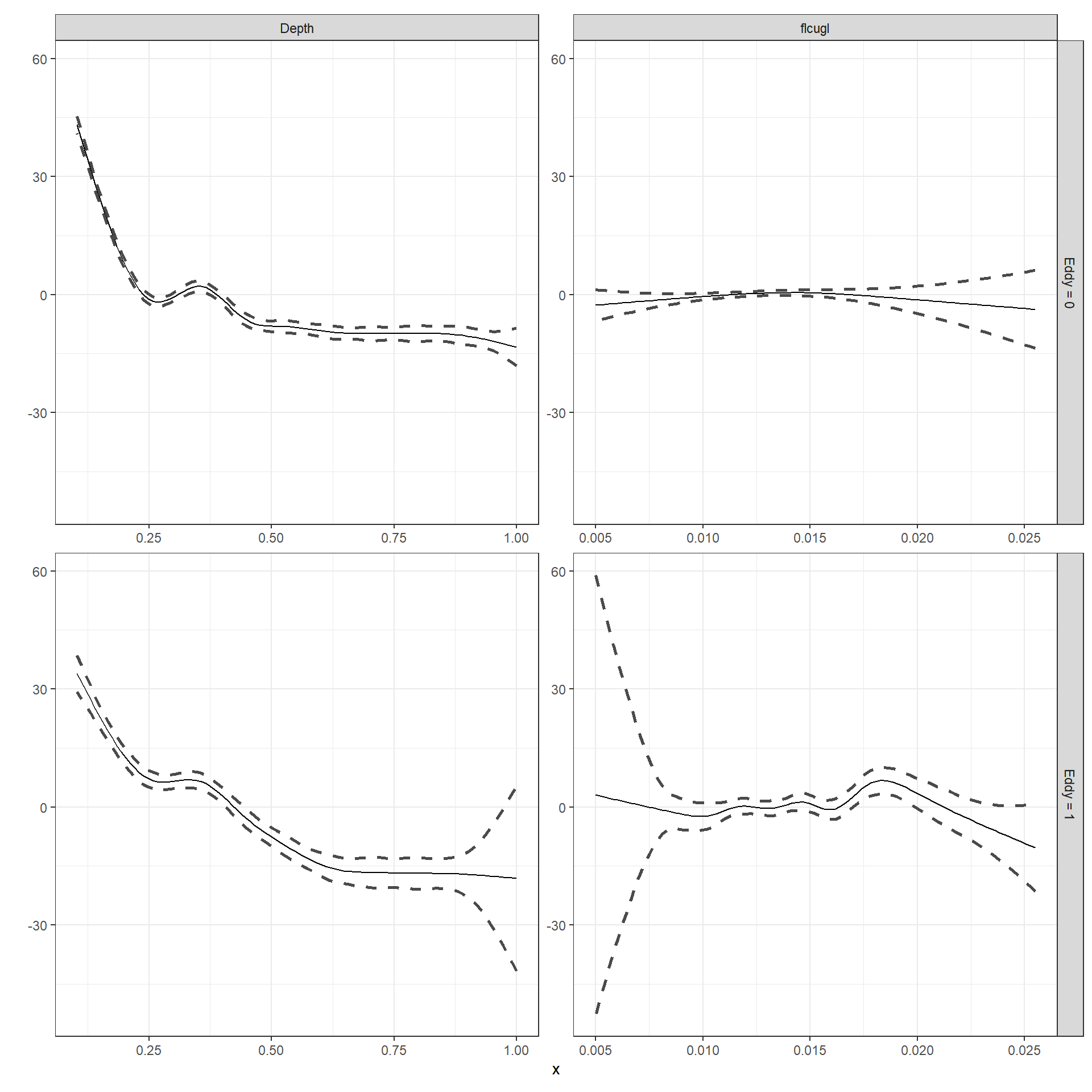
図3.24: Estimated smoothers for mM3_11_e.
References
AICは簡単に言えばより予測の良い(≠ 当てはまりが良い)モデルを選ぶための基準で、低いほど良い。↩︎