9 Marcov Chain Monte Carlo
9.1 Good King Marcov and his island kingdom
10の島からなる諸島がある。それぞれの島は2つの島に隣接しており、全体で円になっている。各島は面積が異なり、それに比例して人口も異なる。面積と人口は1つめの島から順に2倍、3倍、…10倍になっている(つまり、1つめの島の大きさと人口が1だとすれば、10個目の島はそれぞれ10である)。
さて、この諸島の王様は1週間ごとに島々を訪れるが、その際には隣接している島にしか移動できない。王様は各島を人口比率に応じて訪れたいが、訪問計画を長期的に策定するのは面倒である。そこで、彼の側近は以下の方法で島を訪れることを提案した。この方法に従えば、各島に訪れる頻度が人口比率に一致する。ここではこの方法をMetropolis algorithmと呼ぶ。
- 毎週王様はその島にとどまるか、隣接するいずれかの島に移動するかをコインを投げて決める。
- もしコインが表なら、王様は時計回りに隣の島に移動することを考える。一方コインが裏なら、反時計回りに移動することを考える。ここで、提案された島をproposal islandとする。
- 王様はporposal islandの大きさだけ(7つめの島にいるなら7個)貝殻を集める。また、現在いる島の大きさだけ同様に石を集める。
- もし貝殻の数が石よりも多ければ、王様はproposal islandへ移動する。一方で石の数の方が多い場合、王様は集めた石から貝殻と同数の石を捨てる(例えば石が6つ、貝殻が4つなら、手元には\(6-4=2\)個の石が残る)。その後、残された石と貝殻をカバンに入れ、王様はランダムにそのうちの一つを引く。もしそれが貝殻ならばproposal islandに移動し、石ならば今いる島に留まる。
この方法は一見奇妙だが、長期間繰り返していくと非常にうまくいく。以下でシミュレーションしてみよう。
set.seed(9)

num_weeks <- 1e6
positions <- rep(0, num_weeks)
current <- 10

## アルゴリズムの記述
for(i in 1:num_weeks){
  positions[i] <- current
  proposal <- current + sample(c(-1,1), size=1)

  if(proposal <1)  proposal <- 10
  if(proposal >10) proposal <- 1

  prob_move <- proposal/current
  current <- ifelse(runif(1) < prob_move, proposal, current)
}
国王の動きを可視化してみる。
tibble(week = 1:1e6,
       island = positions) %>%
  ggplot(aes(x=week, y = island))+
  geom_line(size=1/3)+
  coord_cartesian(xlim = c(0,500))+
  labs(title = "Behold the Metropolis algorithm in action!",
       subtitle = "The dots show the king's path over the first 500 weeks.")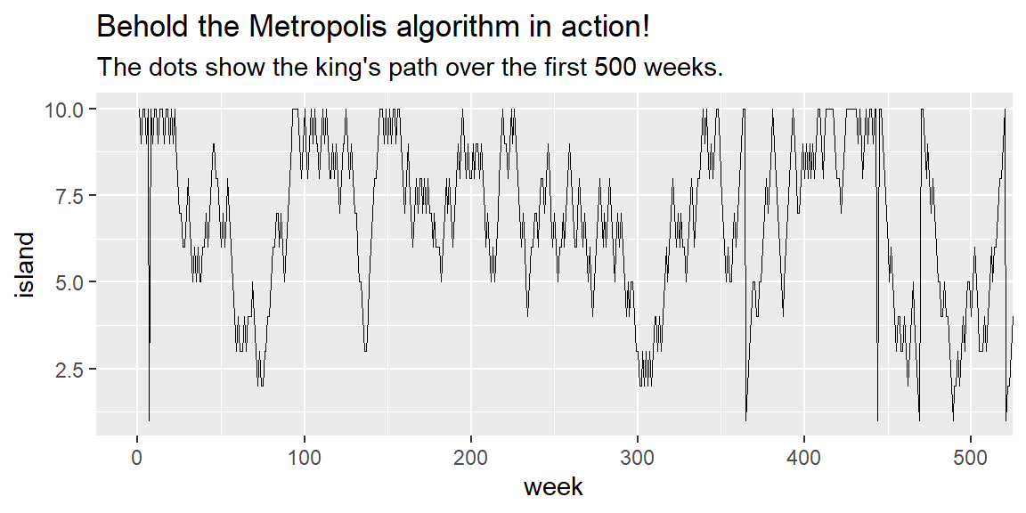
各島を訪れた回数を見てみると以下のようになり、人口に応じて訪れていることが分かる。
tibble(week = 1:1e6,
       island = positions) %>%
  mutate(island = factor(island)) %>%
  ggplot(aes(x=island))+
  geom_bar()+
  labs(title = "Old Metropolis shines in the long run.",
       subtitle = "Sure enough, the time the king spent on each island\nwas proportional to its population size.")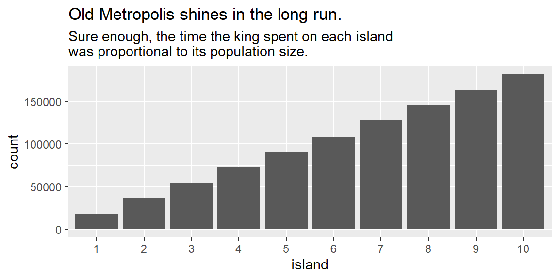
島を訪れている比率はおよそ人口通りになる。このアルゴリズムは、隣の島だけでなく全ての島への移動が可能であっても同様に機能する。
tibble(week = 1:1e6,
       island = positions) %>%
  count(island) %>%
  mutate(prop = n/n[1]) %>%
  gt() %>%
  fmt_number("prop",decimals=2) %>%
tab_options(table.align='left')| island | n | prop |
|---|---|---|
| 1 | 18142 | 1.00 |
| 2 | 36232 | 2.00 |
| 3 | 54787 | 3.02 |
| 4 | 72686 | 4.01 |
| 5 | 90272 | 4.98 |
| 6 | 108747 | 5.99 |
| 7 | 127527 | 7.03 |
| 8 | 145756 | 8.03 |
| 9 | 163703 | 9.02 |
| 10 | 182148 | 10.04 |
9.2 Metropolis algorythm
国王が用いたアルゴリズムはMetropolis algorythmの特殊例であり、このアルゴリズムはマルコフ連鎖モンテカルロ法の一つである。この方法は未知の分布からサンプルを収集するために用いられる。本章では、Metropolis algorythmの改良版であるGibbs samplingについて概説する。
9.2.1 Gibbs sampling
上記のアルゴリズムでは次の島への移動の提案はランダムに(コインによって)行われていたが、より効率よくサンプリングをするためには事後確率に応じて提案が行われる必要がある。そのようなアルゴリズムの一つがGibbs samplingである。
Gibbs samplingはconjugate pairsと呼ばれる特定の事前分布と尤度の組み合わせを用いる方法で、JAGSやBUGSで実装されている。
9.2.2 High-dimentional problem
Gibbs samplingはconjugate pairsが複雑なモデルになると使えなかったり、非効率になったりするという問題点がある。例えば、パラメータ数が多いモデルではパラメータ間に相関がみられることが多く、そのような場合に上手くサンプリングが行えない。
また、concentration of measureという問題によって、パラメータ数が多くなるほどサンプリングは困難になる。まず、あるパラメータの組み合わせの最頻値からの距離を考える。このとき、パラメータ数が多くなるほど、最頻値から離れた距離にあるパラメータの組み合わせが最も多くなってしまう。そのため、パラメータ数が多いほど、最頻値からサンプリングされる確率が低くなってしまう。
以下がシミュレーションである。パラメータ数が増えるにつれて、最頻値(この場合は全てのパラメータが0のとき)から離れたところにあるものが一番多くなることが分かる。
## パラメータ数に応じて各点の距離を計算する関数

concentration_sim <- function(d = 1, t = 1e3, seed = 9) {

  set.seed(seed)

  y <- rethinking::rmvnorm(t, rep(0, d), diag(d))
  rad_dist <- function(y) sqrt(sum(y^2))
  rd <- sapply(1:t, function(i) rad_dist( y[i, ]))

}

## パラメータ数が1, 10, 100, 1000のとき

d <-
  tibble(d = c(1, 10, 100, 1000)) %>%
  mutate(con = purrr::map(d, concentration_sim)) %>%
  unnest(con) %>%
  mutate(`# dimensions` = factor(d))

d  %>%
  ggplot(aes(x = con, fill = `# dimensions`)) +
  geom_density(size = 0, alpha = 3/4)+
  xlab("Radial distance from mode") +
  theme(legend.position = c(.7, .625))+
  theme_classic()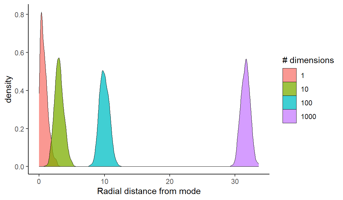
9.3 Hamiltonian Monte Carlo
Hamiltonian Monte Carlo(HMC)法はGibbs samplingなどよりも効率的にサンプリングができるアルゴリズムで、パラメータ数が多くなっても他のアルゴリズムに比べてうまく推定ができる。
9.3.1 Another probable
ここで、またある国を考える。この国の領土は南北に伸びる狭い谷に広がっており、国民は標高と反比例して分布している(高い場所ほど人口が少ない)。さて、この国の国王も国民の人口比率に応じて国中を訪れなければいけないとする。彼の側近のHamiltonは以下のアルゴリズムに従えばうまくいくことを提案した。
- 国王の車はまずランダムな方向にランダムな運動量で動き出す。車は坂道を上がると速度を落とし、やがて運動量の減少とともに坂道を下ってまた加速していく。
- 一定時間後に車を止めて国民にあいさつをする。
- (1)と(2)を繰り返す。
この規則に従うとき、長期的に見れば車がある場所を訪れる頻度は標高に反比例する。この方法はサンプル内の自己相関が低くなるので、分布の幅広い範囲を探索することができる。この方法は諸島では採用できない。なぜならこの方法は国土が連続的であること(=パラメータが連続変数であること)を前提としているからである。
2つのパラメータで簡単なシミュレーションを行う。ここでは以下の統計モデルを用いる。
\[ \begin{aligned} x_{i} &\sim Normal(\mu_{x},1) \\ y_{i} &\sim Normal(\mu_{y},1) \\ \mu_{x} &\sim Normal(0,0.5) \\ \mu_{y} &\sim Normal(0,0.5) \end{aligned} \]
HMCでは、2つの関数と2つの設定によって動く。まず一つ目は対数事後確率であり、以下のようになる(ベイズの定理の分子)。これは、上記の例でいうと標高を表す。
\[
U = \sum_{i} logp(y_{i}|\mu_{y},1) + \sum_{i} logp(x_{i}|\mu_{x},1) + logp(\mu_{y}|0.0.5) + logp(\mu_{x}|0.0.5)
\]
続いて、もう一つ必要な関数は傾きであり、上記の式を\(\mu_{x}\)と\(\mu_{y}\)について偏微分したものに相当する。\(\frac{\partial logN(y|a,b)}{\partial a} = \frac{y-a}{b^2}\)なので、
\[
\begin{aligned}
\frac{\partial U}{\partial \mu_{x}} &= \frac{\partial logN(x|\mu_{x},1)}{\partial \mu_{x}} + \frac{\partial logN(\mu_{x}|0,0.5)}{\partial \mu_{x}} = \sum_{i} \frac {x_{i} - \mu_{x}}{1^2} + \frac {0-\mu_{x}}{0.5^2} \\
\frac{\partial U}{\partial \mu_{y}} &= \frac{\partial logN(y|\mu_{y},1)}{\partial \mu_{y}} + \frac{\partial logN(\mu_{y}|0,0.5)}{\partial \mu_{y}} = \sum_{i} \frac {y_{i} - \mu_{y}}{1^2} + \frac {0-\mu_{y}}{0.5^2}
\end{aligned}
\]
必要な2つの設定は、step sizeとleapfrog stepsの数(何ステップに1回サンプリングするか)である。効率的にサンプリングするためには、これらを適切に設定することが必要であるが、通常はソフトウェアが設定してくれる。stanでは、warmup期間中にこのチューニングが行われる。また、NUTSというアルゴリズムによって、運動ベクトルが大きく変わった時にサンプリングを行うことで、同じ場所からばかりサンプリングが行われることを防いでいる。
9.4 Easy HMC: ulam brm()
Chapter8の地形とGDPに関するデータについて再び検討する。
## データ読み込み
data(rugged)
d <- rugged

## 標準化(GDPは対数をとる)
d %>%
  dplyr::select(country,cont_africa,rugged,rgdppc_2000) %>% filter(complete.cases(rgdppc_2000)) %>%
  mutate(G = log(rgdppc_2000)/mean(log(rgdppc_2000),
                                   na.rm=T),
         R = rugged/max(rugged),
         A = ifelse(cont_africa=="1","1","2")) %>%
mutate(R_c = R - mean(R))-> d29.4.2 Sampling from posterior
それでは、brmsでモデリングを行う。
b9.1 <-
  brm(data = d2,
      family = gaussian,
      formula = bf(G ~ 0 + a + b*R_c,
                   a ~ 0 + A,
                   b ~ 0 + A,
                   nl = TRUE),
      prior = c(prior(normal(1, 0.1), class = b, nlpar = a),
                prior(normal(0, 0.3), class = b, nlpar = b),
                prior(exponential(1), class=sigma)),
      seed = 9, chain =1, cores=1,
      backend = "cmdstanr",
      file = "output/Chapter9/b9.1")

#posterior_summary(b9.1) %>%
  #data.frame() %>%
  #rownames_to_column(var ="parameters") %>%
  #filter(parameters != "lp__") %>%
  #gt()

posterior_samples(b9.1) %>%
  pivot_longer(-lp__, names_to = "parameters") %>%
  group_by(parameters) %>%
  mean_hdi(value, .width = .89) %>%
gt()| parameters | value | .lower | .upper | .width | .point | .interval |
|---|---|---|---|---|---|---|
| b_a_A1 | 0.8864752 | 0.860290836 | 0.90806460 | 0.89 | mean | hdi |
| b_a_A2 | 1.0504113 | 1.033940994 | 1.06580555 | 0.89 | mean | hdi |
| b_b_A1 | 0.1260194 | 0.005795189 | 0.25055026 | 0.89 | mean | hdi |
| b_b_A2 | -0.1446658 | -0.231614404 | -0.04967538 | 0.89 | mean | hdi |
| lprior | 2.1821531 | 1.804216122 | 2.54075927 | 0.89 | mean | hdi |
| sigma | 0.1116524 | 0.101538272 | 0.12156657 | 0.89 | mean | hdi |
#rhat(b9.1)9.4.3 Sampling again in parallel
次は、4つのchainで回してみる。
b9.1b <-
  update(b9.1,
         chains = 4, cores=4,
         seed=9, file = "output/Chapter9/b9.1b")

posterior_samples(b9.1b) %>%
  pivot_longer(-lp__, names_to = "parameters") %>%
  group_by(parameters) %>%
  mean_hdi(value, .width = .89) %>%
gt()| parameters | value | .lower | .upper | .width | .point | .interval |
|---|---|---|---|---|---|---|
| b_a_A1 | 0.8866523 | 0.86013454 | 0.91021227 | 0.89 | mean | hdi |
| b_a_A2 | 1.0507625 | 1.03399223 | 1.06591912 | 0.89 | mean | hdi |
| b_b_A1 | 0.1321000 | 0.01681887 | 0.25173934 | 0.89 | mean | hdi |
| b_b_A2 | -0.1425208 | -0.23471392 | -0.05644302 | 0.89 | mean | hdi |
| lprior | 2.1793178 | 1.80629736 | 2.54256135 | 0.89 | mean | hdi |
| sigma | 0.1116139 | 0.10205780 | 0.12163415 | 0.89 | mean | hdi |
全ての結果
print(b9.1b)## Family: gaussian
## Links: mu = identity; sigma = identity
## Formula: G ~ 0 + a + b * R_c
## a ~ 0 + A
## b ~ 0 + A
## Data: d2 (Number of observations: 170)
## Draws: 4 chains, each with iter = 2000; warmup = 1000; thin = 1;
## total post-warmup draws = 4000
##
## Population-Level Effects:
## Estimate Est.Error l-95% CI u-95% CI Rhat Bulk_ESS Tail_ESS
## a_A1 0.89 0.02 0.86 0.92 1.00 4788 3163
## a_A2 1.05 0.01 1.03 1.07 1.00 4423 3086
## b_A1 0.13 0.07 -0.02 0.28 1.00 4279 2983
## b_A2 -0.14 0.06 -0.25 -0.03 1.00 4892 2828
##
## Family Specific Parameters:
## Estimate Est.Error l-95% CI u-95% CI Rhat Bulk_ESS Tail_ESS
## sigma 0.11 0.01 0.10 0.12 1.00 4850 2996
##
## Draws were sampled using sampling(NUTS). For each parameter, Bulk_ESS
## and Tail_ESS are effective sample size measures, and Rhat is the potential
## scale reduction factor on split chains (at convergence, Rhat = 1).#以下でも同じ出力
#summary(b9.1b)
#show(b9.1)モデル式
b9.1b$formula## G ~ 0 + a + b * R_c
## a ~ 0 + A
## b ~ 0 + A事前分布
b9.1b$prior %>%
print()## prior class coef group resp dpar nlpar lb ub source
## normal(1, 0.1) b a user
## normal(1, 0.1) b A1 a (vectorized)
## normal(1, 0.1) b A2 a (vectorized)
## normal(0, 0.3) b b user
## normal(0, 0.3) b A1 b (vectorized)
## normal(0, 0.3) b A2 b (vectorized)
## exponential(1) sigma 0 user#以下でも同じ
#prior_summary(b9.1b)9.4.4 Visualization
各パラメータの事後分布と変数間の相関はpairs()とvcoc()で確認できる。ただし、\(\sigma\)は入らない。
pairs(b9.1b,
off_diag_args = list(size = 1/5, alpha = 1/5))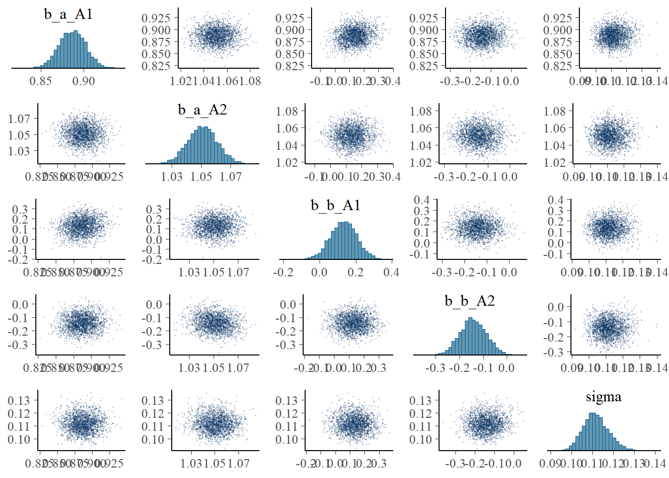
#vcov(b9.1b, correlation=T) %>%
# round(2) GGallyパッケージの`ggpairs()’を使えば、\(\sigma\)も入れて可視化可能。
library(GGally)
posterior_samples(b9.1b) %>%
dplyr::select(-lp__) %>%
ggpairs()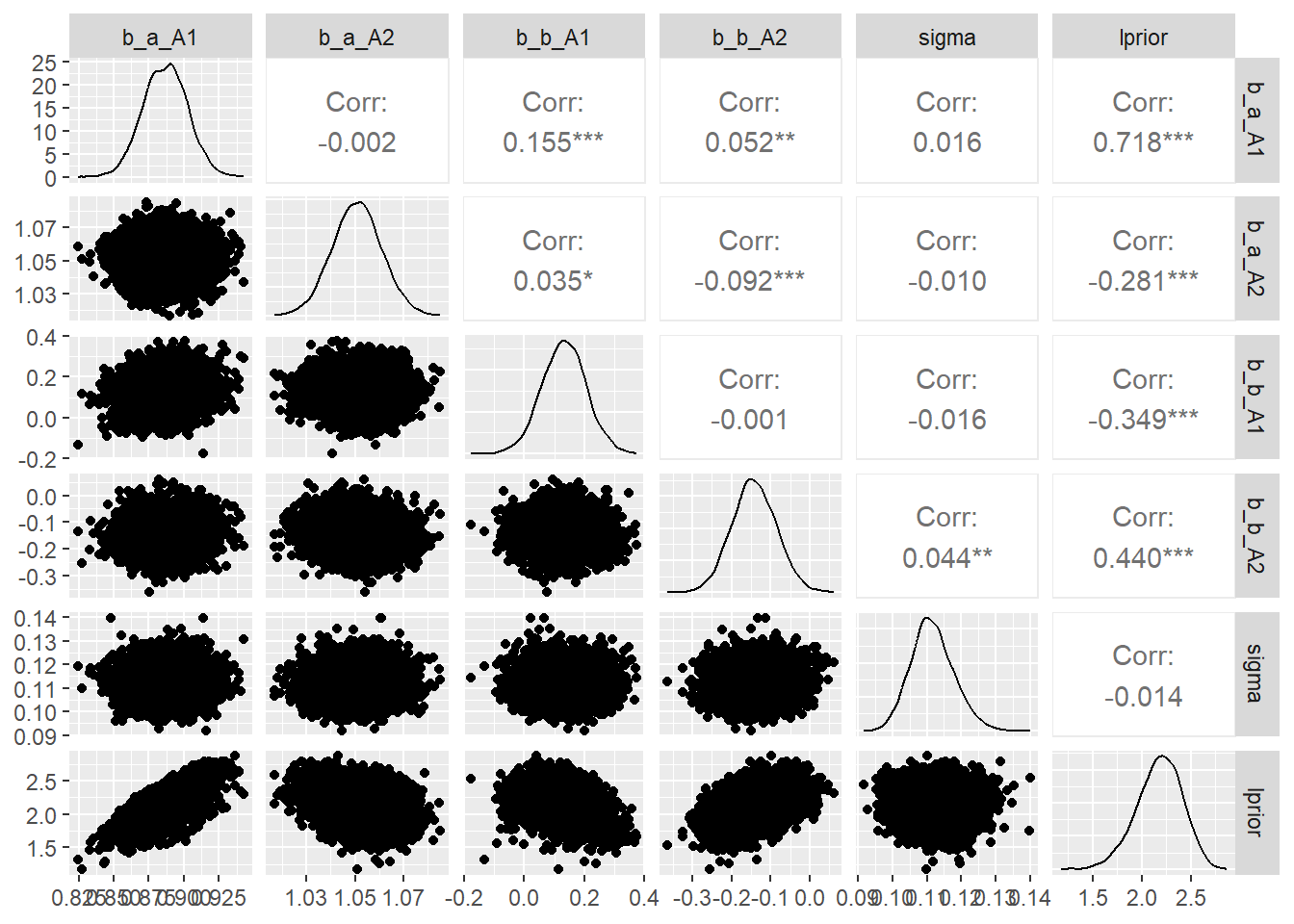
9.4.5 Checking the chain
収束を診断する際には、まずトレースプロットを確認する。
bayesplotパッケージが便利である。
## brms
plot(b9.1b)
## bayesplot
library(bayesplot)
post <-
posterior_samples(b9.1b, add_chain =TRUE) #chainの情報を残す
mcmc_trace(post[,c(1:5,7)],
facet_args = list(ncol=3),
size=.15) 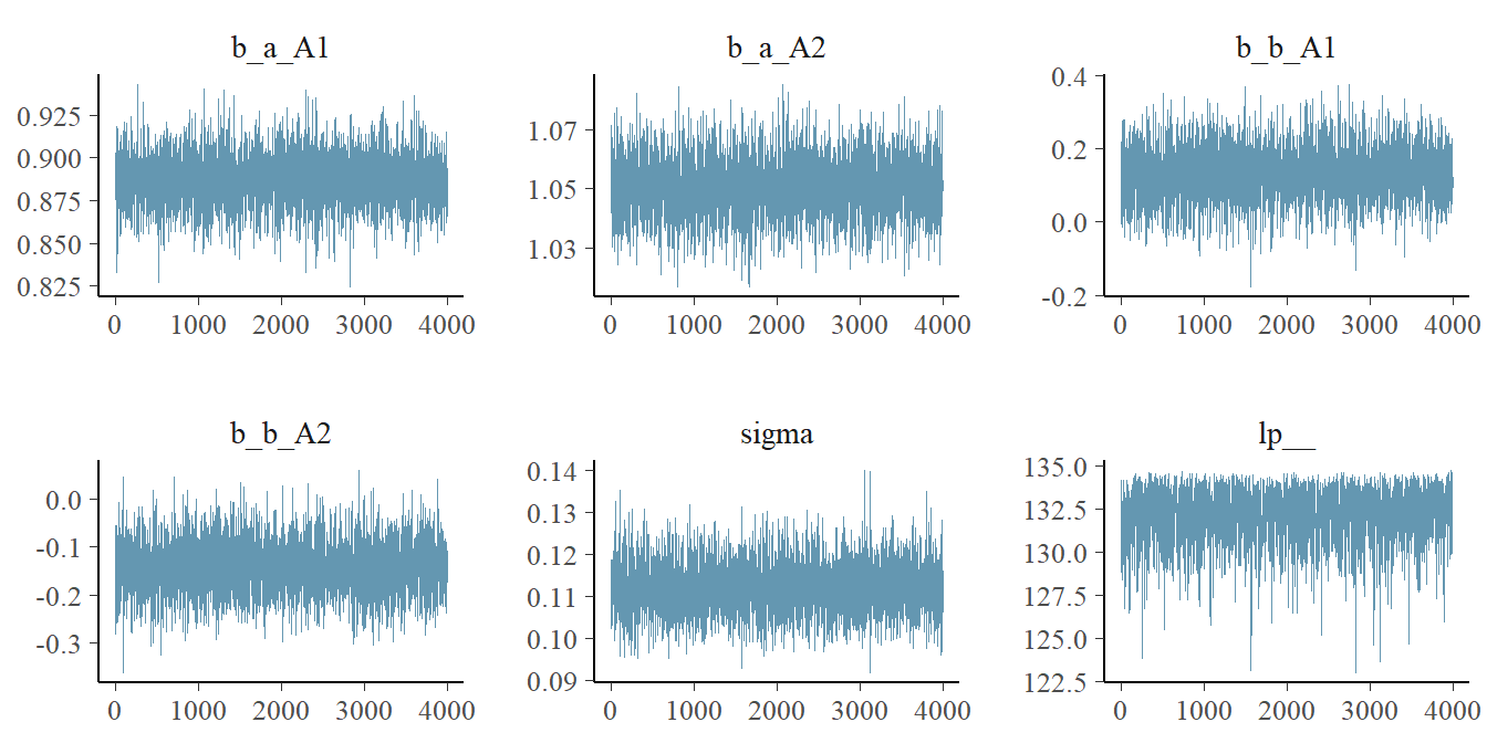
自己相関を確認する。
post %>%
mcmc_acf(pars = vars(1:5),
lags=5)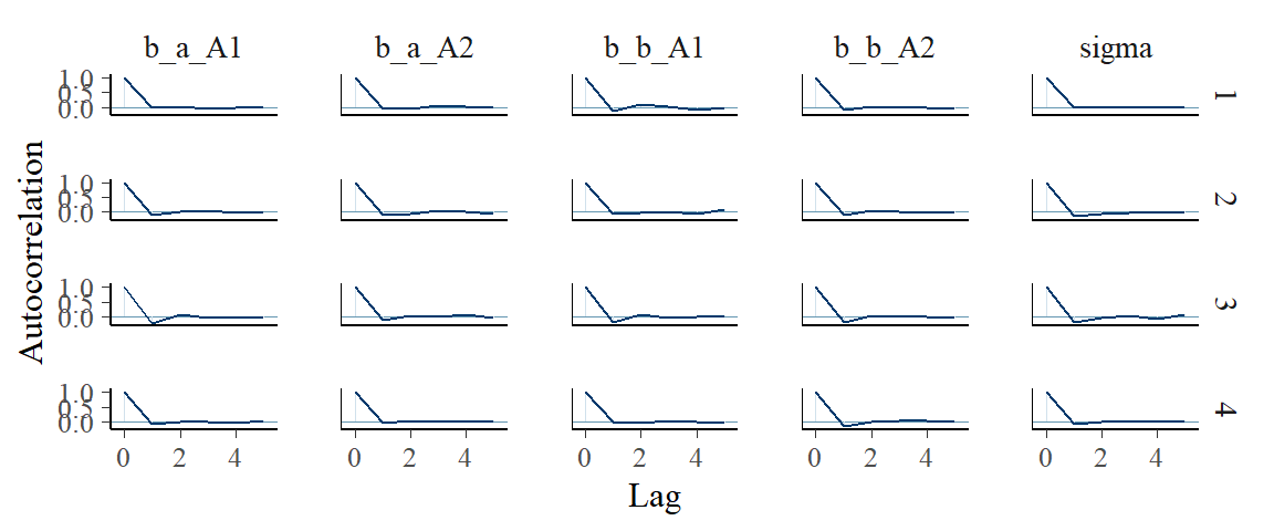
warmup期間のサンプルを含む場合には、ggmcmcパッケージを用いるとよい。
library(ggmcmc)
ggs(b9.1b) %>%
mutate(chain = factor(Chain)) %>%
ggplot(aes(x=Iteration, y=value))+
annotate(geom = "rect",
xmin = 0, xmax = 1000, ymin = -Inf, ymax = Inf,
fill = "grey",
alpha = 3/6, size = 0) +
geom_line(aes(color = chain),
size = .15)+
theme_classic()+
theme(strip.background = element_blank(),
legend.position = c(.75, .18))+
facet_wrap(~Parameter, scales = "free_y")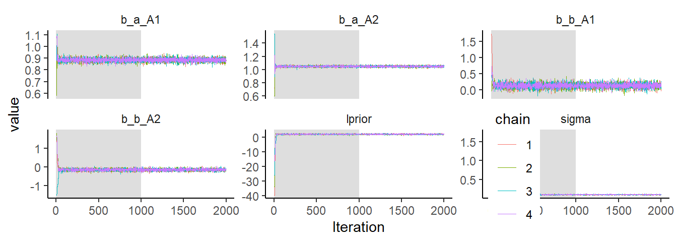
最初の50サンプル
ggs(b9.1b) %>%
mutate(chain = factor(Chain)) %>%
ggplot(aes(x=Iteration, y=value))+
annotate(geom = "rect",
xmin = 0, xmax = 1000, ymin = -Inf, ymax = Inf,
fill = "grey",
alpha = 3/6, size = 0) +
geom_line(aes(color = chain),
size = .15)+
theme_classic()+
theme(strip.background = element_blank(),
legend.position = c(.75, .18))+
coord_cartesian(xlim=c(0,50))+
facet_wrap(~Parameter, scales = "free_y")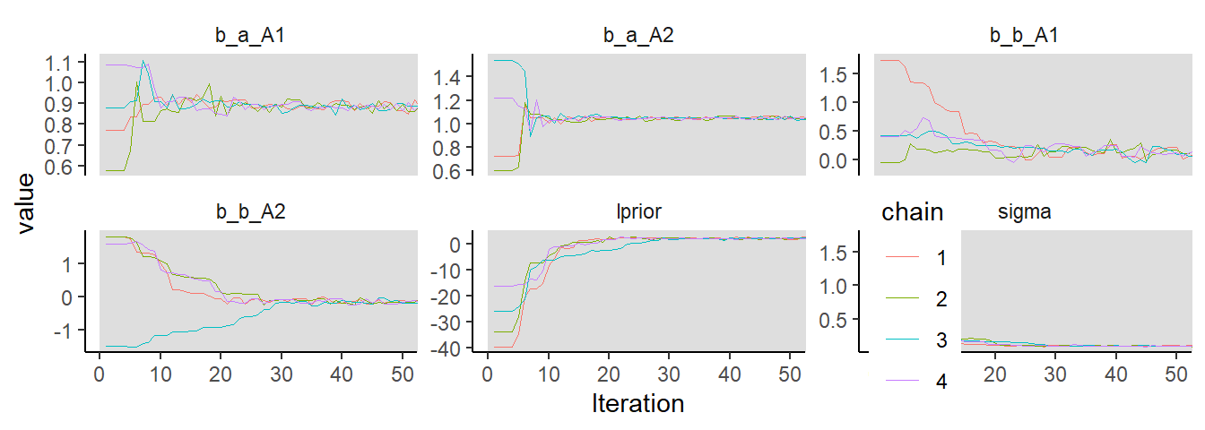
トレースプロットの診断では、以下の3つの基準を満たしているかを確認する。
- stationarity
chainがある一定の範囲から安定して得られているか。別の言い方をすると、サンプルの平均値が最初から最後まで安定しているか。
- good mixing
chainが全ての範囲から素早く探索できているか。
- convergence
それぞれのchainが同じ範囲に収まっているか。
もうひとつ収束を確認する方法としてtrace rank plot、もしくはtrank plotをみるというものがある。これは、サンプルを小さい方から順に1, 2, 3,…,Nというように順位づけ、chainごとにヒストグラムを描くというもの。もしうまく収束できていれば、各ヒストグラムは似たような形になり、重複するはず。
post %>%
mcmc_rank_overlay(pars = vars(1:5))+
coord_cartesian(ylim=c(25,NA))+
theme(legend.position = c(.75,.2))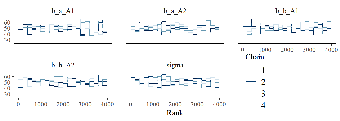
9.5 Care and feeding of your Marcov chain
HMCのすぐれたところは、その効率性だけでなく、もしサンプリングがうまくいっていないときにそれが簡単にわかるということである。以下で、サンプリングがうまくいっていない場合を見ていこう。
9.5.1 How many samples do you need
- 重要なのはどのくらい有効サンプル数(自己相関していないマルコフ連鎖の長さ)である。有効サンプルサイズはサンプルに負の自己相関がある場合には、chainの長さよりも大きくなることがありうる。なお、bulk-ESSは事後分布の中心でどの程度有効サンプルが得られているかを評価している一方で、tail-ESSはより広い区間についてのものであるので、区間推定を行う場合にはtail-ESSに着目する。
- 何を知りたいかによって必要なサンプルサイズは異なる。もし事後分布の平均を知りたいだけであればそこまで多くのサンプルを必要としないが、より広い範囲(例えば、99%信用区間など)について調べたければ、より多くのサンプルを必要とする。一般的に、平均の推定値を知りたいだけならば、有効サンプルサイズは200程度でよい。また、事後分布が正規分布に近似できれば、分布の分散を推定すればうまく区間推定ができるが、偏りのある分布では区間推定のために多くのサンプルを必要とする。
9.5.2 How many chains do we need
- デバッグをする場合には、まず1つを回してうまくいくか確認する。
- その後、終息の診断をするときには1つ以上のchainが必要。その場合、3~4個で十分。
- 最後に(上手く収束することが分かった後に)推定をする際には1つでも構わない。2つ以上でもよいが、全てのchainでwarmupすることになるので、効率は悪くなる。
収束の判断について詳しくは以下のリンクを参照。 Visual MCMC diagnostics using the bayesplot package
9.5.3 Taming and wild chain
極端に小さい(大きい)値からサンプリングをしてしまっている例を見ていく。これは事前分布が広すぎる場合にしばしば起きる。
b9.2 <-
brm(data = list(y=c(-1,1)),
family=gaussian,
y~1,
prior = c(prior(normal(0, 1000), class = Intercept),
prior(exponential(0.0001), class = sigma)),
iter = 2000, warmup = 1000, chains = 3,
backend = "cmdstanr",
seed = 9,
file = "output/Chapter9/b9.2")エラーがかなり出ている。また、結果もあり得ない値になっている。有効サンプルサイズもかなり小さい。
print(b9.2)## Warning: There were 433 divergent transitions after
## warmup. Increasing adapt_delta above 0.8 may help. See
## http://mc-stan.org/misc/warnings.html#divergent-transitions-after-warmup## Family: gaussian
## Links: mu = identity; sigma = identity
## Formula: y ~ 1
## Data: list(y = c(-1, 1)) (Number of observations: 2)
## Draws: 3 chains, each with iter = 2000; warmup = 1000; thin = 1;
## total post-warmup draws = 3000
##
## Population-Level Effects:
## Estimate Est.Error l-95% CI u-95% CI Rhat Bulk_ESS Tail_ESS
## Intercept 4.46 332.87 -782.85 767.68 1.01 604 388
##
## Family Specific Parameters:
## Estimate Est.Error l-95% CI u-95% CI Rhat Bulk_ESS Tail_ESS
## sigma 554.99 1407.42 26.10 3613.65 1.02 108 86
##
## Draws were sampled using sample(hmc). For each parameter, Bulk_ESS
## and Tail_ESS are effective sample size measures, and Rhat is the potential
## scale reduction factor on split chains (at convergence, Rhat = 1).nuts_param()関数をつかえば診断情報を調べることができる。
3000サンプルの内282個でdivergent transitionが起きていることが分かる。
## 項目
nuts_params(b9.2) %>%
distinct() %>%
datatable()## divergentについて
nuts_params(b9.2) %>%
filter(Parameter == "divergent__") %>%
count(Value)## Value n
## 1 0 2567
## 2 1 433pairs()を用いて診断結果を図示できる。赤い点がdivergent transitionが起きているサンプル。
※ 現在うまく出力されない。
pairs(b9.2,
off_diag_args = list(size = 1/4))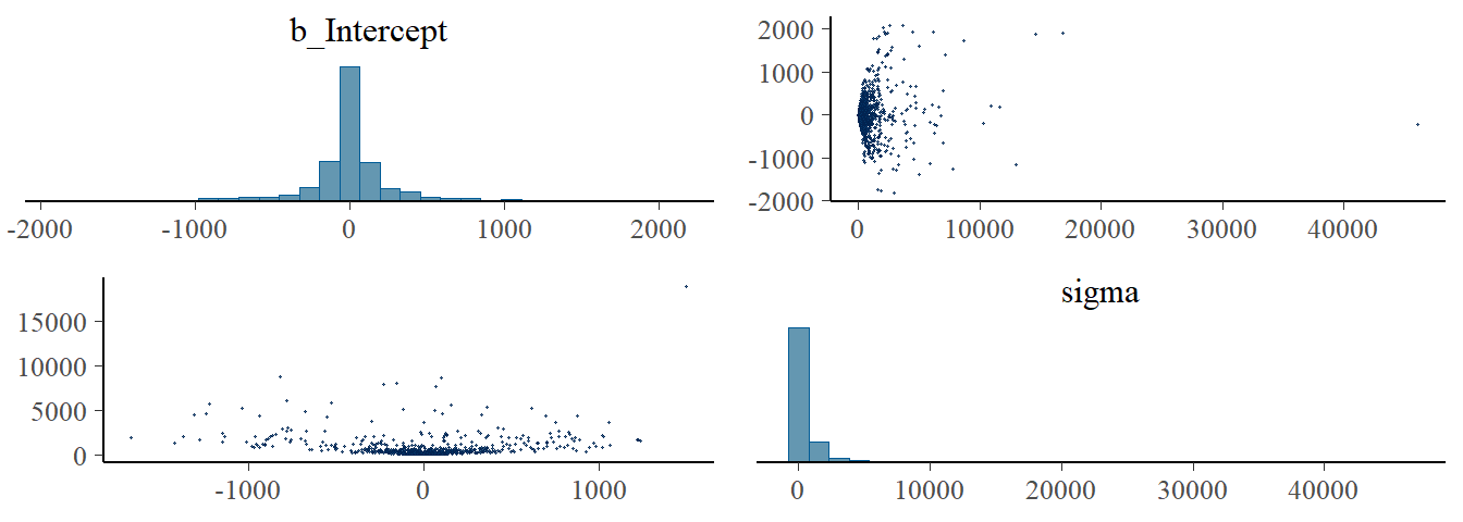
chainを確認しても、うまく収束していないことが分かる。
post <- posterior_samples(b9.2, add_chain = TRUE)
p1 <- post %>%
mcmc_trace(pars = vars(1:2),
size=.25)
p2 <-
post %>%
mcmc_rank_overlay(pars = vars(1:2))
((p1/p2)&
theme(legend.position="none")&
plot_annotation(subtitle = "These chains are not healthy"))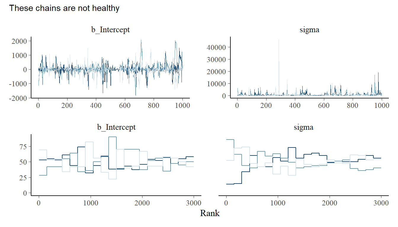
弱情報事前分布を用いることで、この問題を解決できる。
b9.3 <-
brm(data = list(y=c(-1,1)),
family=gaussian,
y~1,
prior = c(prior(normal(1, 10), class = Intercept),
prior(exponential(1), class = sigma)),
iter = 2000, warmup = 1000, chains = 3,
seed = 9,
backend = "cmdstanr",
file = "output/Chapter9/b9.3")
print(b9.3)## Family: gaussian
## Links: mu = identity; sigma = identity
## Formula: y ~ 1
## Data: list(y = c(-1, 1)) (Number of observations: 2)
## Draws: 3 chains, each with iter = 2000; warmup = 1000; thin = 1;
## total post-warmup draws = 3000
##
## Population-Level Effects:
## Estimate Est.Error l-95% CI u-95% CI Rhat Bulk_ESS Tail_ESS
## Intercept 0.03 1.16 -2.28 2.46 1.00 1256 1050
##
## Family Specific Parameters:
## Estimate Est.Error l-95% CI u-95% CI Rhat Bulk_ESS Tail_ESS
## sigma 1.54 0.81 0.61 3.63 1.00 989 979
##
## Draws were sampled using sample(hmc). For each parameter, Bulk_ESS
## and Tail_ESS are effective sample size measures, and Rhat is the potential
## scale reduction factor on split chains (at convergence, Rhat = 1).divergent transitionも起きていない。
pairs(b9.3,
np = nuts_params(b9.3),
off_diag_args = list(size = 1/4))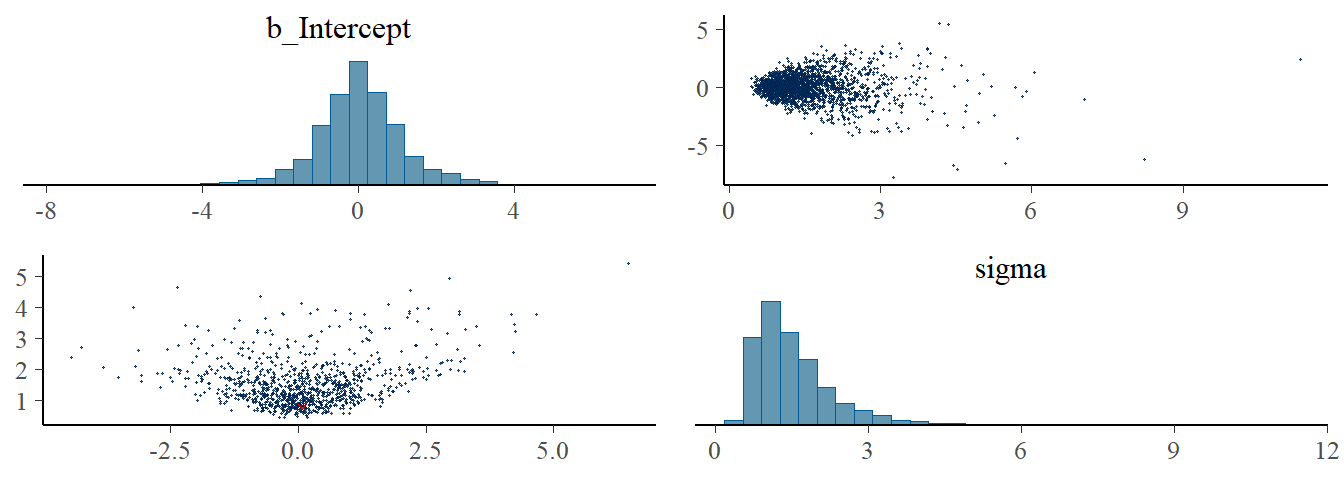
traceplotも概ね問題なさそう。
post_weekprior <- posterior_samples(b9.3, add_chain = TRUE)
p3 <- post_weekprior %>%
mcmc_trace(pars = vars(1:2),
size=.25)
p4 <-
post_weekprior %>%
mcmc_rank_overlay(pars = vars(1:2))
((p3/p4)&
theme(legend.position="none")&
plot_annotation(subtitle = "Weakly informative priors cleared up the condition right away"))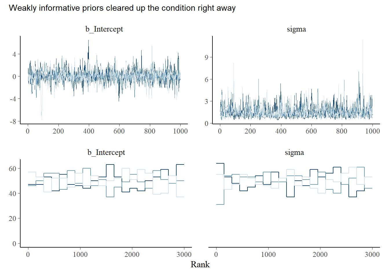
事前分布と事後分布を図示してみる。
事前分布に少し情報を与えただけで、推定がうまくいくことが分かる。
post_weekprior %>%
dplyr::select(b_Intercept) %>%
ggplot(aes(x=b_Intercept))+
geom_density(trim = T, color="navy")+
geom_line(data=tibble(x=seq(-15,15,length.out=50)),
aes(x=x, y=dnorm(x,mean=1,sd=10)),
linetype=2, color="grey26")+
theme_classic()+
theme(aspect.ratio=1)+
xlab(expression(alpha)) ->p5
post_weekprior %>%
dplyr::select(sigma) %>%
ggplot(aes(x=sigma))+
geom_density(trim = T, color="navy")+
geom_line(data=tibble(x=seq(0,10,length.out=50)),
aes(x=x, y=dexp(x,1)),
linetype=2, color = "grey26")+
theme_classic()+
theme(aspect.ratio=1)+
xlab(expression(sigma)) ->p6
p5+p6+
plot_annotation(title = "Prior (dashed) vs posterior (solod) distributions. ")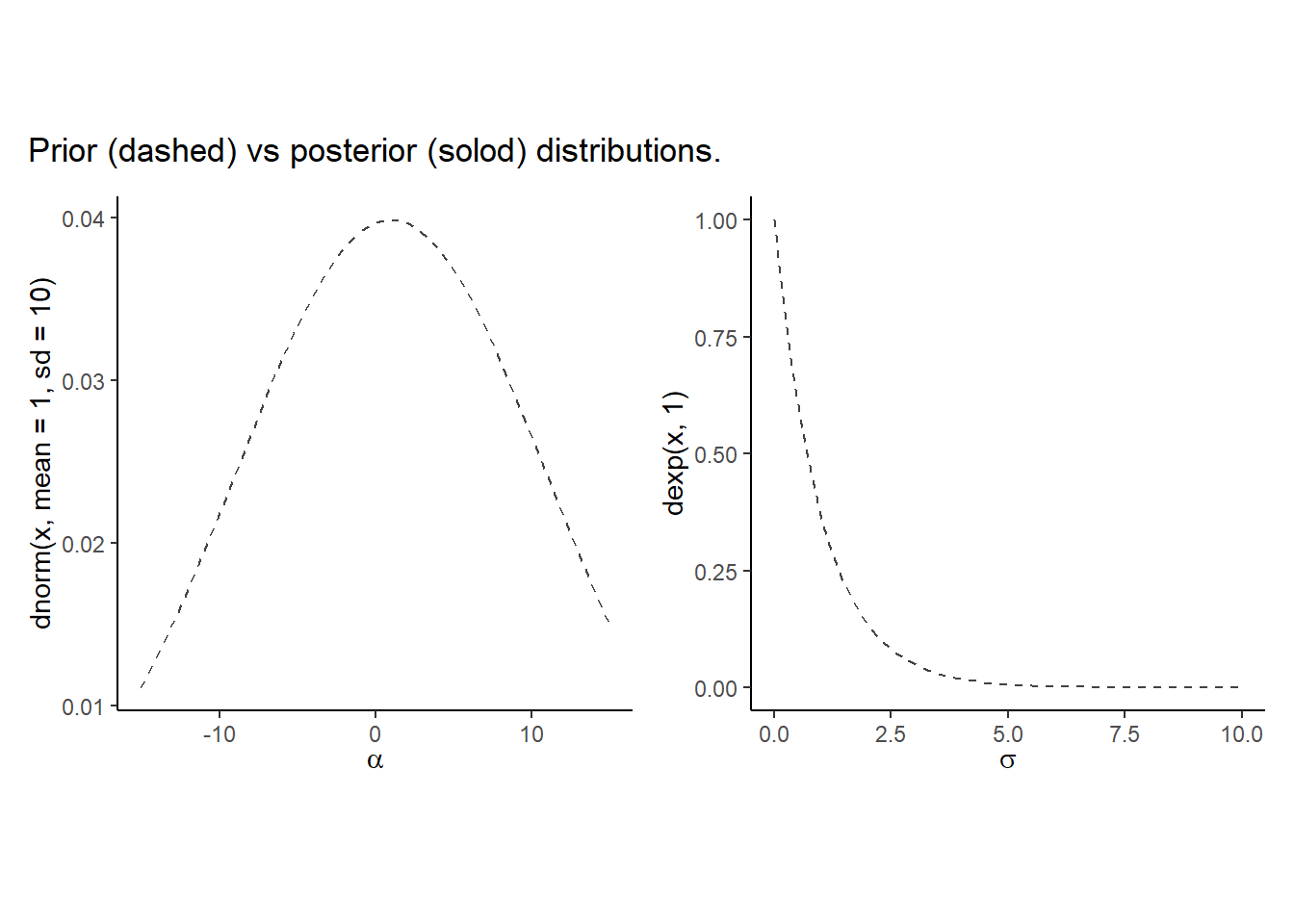
9.5.4 Non-identifiable parameters
識別不能な(一意に定まらない)パラメータがあるモデルを考え、そのときHMCがどのように働いているかを見てみる。
\[
\begin{aligned}
y_{i} &\sim Normal(\mu,\sigma)\\
\mu &= \alpha_{1} + \alpha_{2}\\
\alpha_{1} &\sim Normal(0,1000)\\
\alpha_{2} &\sim Normal(0,1000)\\
\sigma &\sim Exponential(1)
\end{aligned}
\]
set.seed(384)
y <- rnorm(100,0,1)
b9.4 <- brm(
data = list(y = y,
a1 = 1,
a2 = 1),
family=gaussian,
y ~ 0 + a1 + a2,
prior = c(prior(normal(0, 1000), class = b),
prior(exponential(1), class = sigma)),
iter = 2000, warmup = 1000, chains = 3,
seed = 9,
backend = "cmdstanr",
file = "output/Chapter9/b9.4"
)上手く推定ができない。ほとんど有効サンプルがない。
また、上手く収束できていない。
print(b9.4)## Warning: Parts of the model have not converged (some Rhats are > 1.05). Be
## careful when analysing the results! We recommend running more iterations and/or
## setting stronger priors.## Family: gaussian
## Links: mu = identity; sigma = identity
## Formula: y ~ 0 + a1 + a2
## Data: list(y = y, a1 = 1, a2 = 1) (Number of observations: 100)
## Draws: 3 chains, each with iter = 2000; warmup = 1000; thin = 1;
## total post-warmup draws = 3000
##
## Population-Level Effects:
## Estimate Est.Error l-95% CI u-95% CI Rhat Bulk_ESS Tail_ESS
## a1 310.57 590.61 -676.22 1466.19 2.38 4 12
## a2 -310.73 590.61 -1466.48 676.00 2.38 4 12
##
## Family Specific Parameters:
## Estimate Est.Error l-95% CI u-95% CI Rhat Bulk_ESS Tail_ESS
## sigma 1.08 0.08 0.94 1.26 1.15 25 45
##
## Draws were sampled using sample(hmc). For each parameter, Bulk_ESS
## and Tail_ESS are effective sample size measures, and Rhat is the potential
## scale reduction factor on split chains (at convergence, Rhat = 1).chainをみても収束がうまくいっていないのは明らか。
post_UI <- posterior_samples(b9.4, add_chain = TRUE)
post_UI %>%
mcmc_trace(pars = vars(1:3),
size=.25)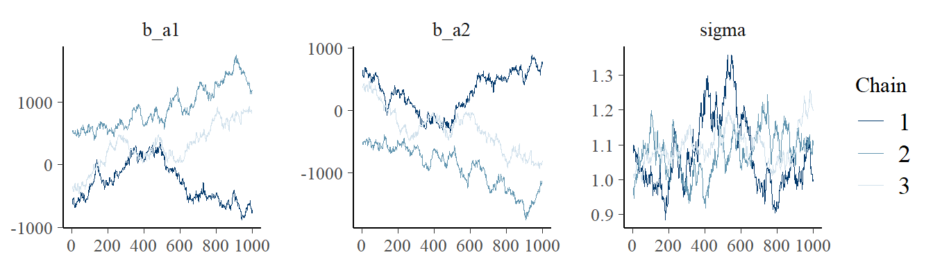
post_UI %>%
mcmc_rank_overlay(pars = vars(1:3))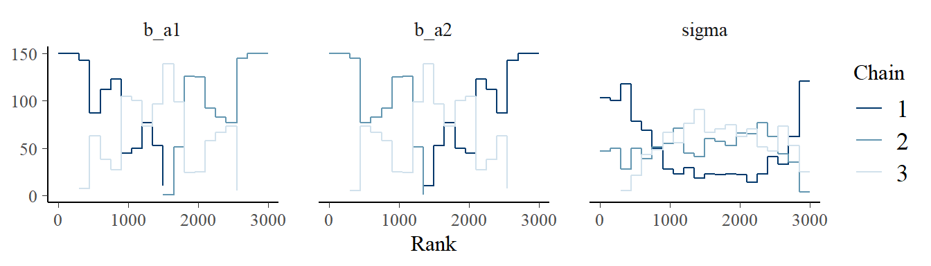
再び、弱情報事前分布を設定するとうまく推定ができる。
b9.5 <- brm(
data = list(y = y,
a1 = 1,
a2 = 1),
family=gaussian,
y ~ 0 + a1 + a2,
prior = c(prior(normal(0, 10), class = b),
prior(exponential(1), class = sigma)),
iter = 2000, warmup = 1000, chains = 3,
seed = 9,
backend = "cmdstanr",
file = "output/Chapter9/b9.5"
)上手く推定ができている。a1とa2の係数は一意に定まらないが、その合計はうまく推定できる。
print(b9.5)## Family: gaussian
## Links: mu = identity; sigma = identity
## Formula: y ~ 0 + a1 + a2
## Data: list(y = y, a1 = 1, a2 = 1) (Number of observations: 100)
## Draws: 3 chains, each with iter = 2000; warmup = 1000; thin = 1;
## total post-warmup draws = 3000
##
## Population-Level Effects:
## Estimate Est.Error l-95% CI u-95% CI Rhat Bulk_ESS Tail_ESS
## a1 -0.41 6.99 -14.16 12.85 1.00 725 600
## a2 0.24 6.99 -13.11 14.14 1.00 724 597
##
## Family Specific Parameters:
## Estimate Est.Error l-95% CI u-95% CI Rhat Bulk_ESS Tail_ESS
## sigma 1.07 0.08 0.93 1.23 1.00 1164 1072
##
## Draws were sampled using sample(hmc). For each parameter, Bulk_ESS
## and Tail_ESS are effective sample size measures, and Rhat is the potential
## scale reduction factor on split chains (at convergence, Rhat = 1).二つのモデルのtraceplotを比べてみる。
# b9.4
post_b9.4 <- posterior_samples(b9.4, add_chain=TRUE)
p7 <- trace_rank(data = post_b9.4, var = "b_a1", subtitle = "b9.4 (bad priors)")
p8 <- trace_rank(data = post_b9.4, var = "b_a2")
p9 <- trace_rank(data = post_b9.4, var = "sigma")
# b9.4
post_b9.5 <- posterior_samples(b9.5, add_chain=TRUE)
p10 <- trace_rank(data = post_b9.5, var = "b_a1", subtitle = "b9.5 (good priors)")
p11 <- trace_rank(data = post_b9.5, var = "b_a2")
p12 <- trace_rank(data = post_b9.5, var = "sigma")
(p7/p8/p9/p10/p11/p12)&
theme(legend.position = "none")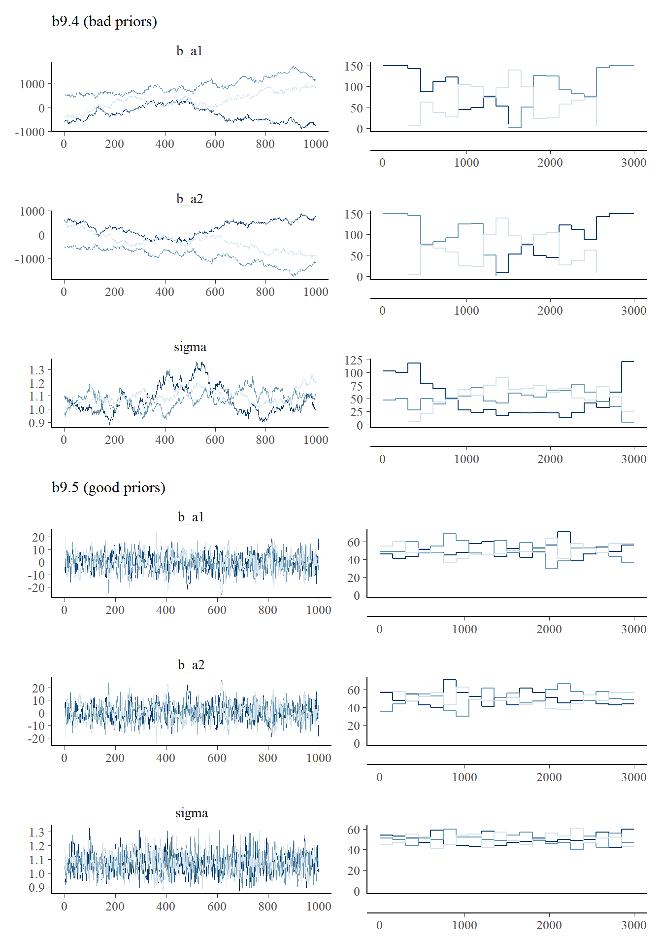
9.6 Practice
9.6.1 9M1
Re-estimate the terrain ruggedness model from the chapter, but now using a uniform prior and an exponential prior for the standard deviation, sigma. The uniform prior should be dunif(0,10) and the exponential should be dexp(1). Do the different priors have any detectable influence on the posterior distribution?
再びGDPと地形の関連についてモデリングするが、今回は標準偏差の事前分布に一様分布を用いる。
b9.1_unif <-
brm(data = d2,
family = gaussian,
formula = bf(G ~ 0 + a + b*R_c,
a ~ 0 + A,
b ~ 0 + A,
nl = TRUE),
prior = c(prior(normal(1, 0.1), class = b, nlpar = a),
prior(normal(0, 0.3), class = b, nlpar = b),
prior(uniform(0,1), class=sigma)),
seed = 9, chain =4, cores=4,
backend = "cmdstanr",
file = "output/Chapter9/b9.1_unif")事後分布にほとんど影響はない。
## Exponential(1)
posterior_summary(b9.1b) %>%
data.frame() %>%
rownames_to_column(var = "parameters") %>%
filter(parameters != "lp__") %>%
gt()| parameters | Estimate | Est.Error | Q2.5 | Q97.5 |
|---|---|---|---|---|
| b_a_A1 | 0.8866523 | 0.015798028 | 0.85643840 | 0.91717842 |
| b_a_A2 | 1.0507625 | 0.010079614 | 1.03083530 | 1.07050915 |
| b_b_A1 | 0.1321000 | 0.073764966 | -0.01533556 | 0.27864973 |
| b_b_A2 | -0.1425208 | 0.056347768 | -0.25179496 | -0.03043489 |
| sigma | 0.1116139 | 0.006185409 | 0.10034831 | 0.12474091 |
| lprior | 2.1793178 | 0.231572347 | 1.69404549 | 2.59457936 |
plot(b9.1b, pars = "sigma")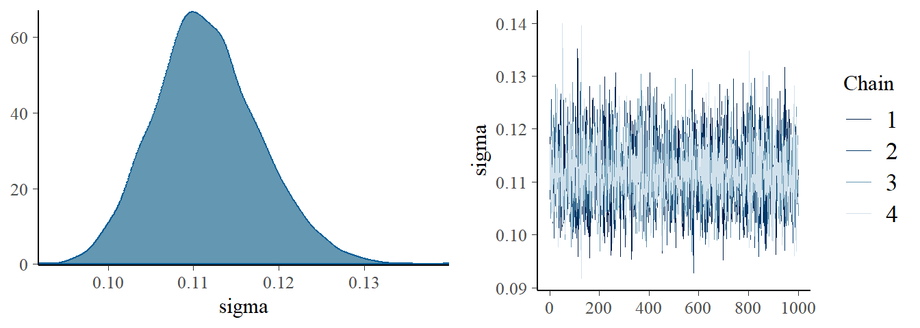
## Uniform(0,1)
posterior_summary(b9.1_unif) %>%
data.frame() %>%
rownames_to_column(var = "parameters") %>%
filter(parameters != "lp__") %>%
gt()| parameters | Estimate | Est.Error | Q2.5 | Q97.5 |
|---|---|---|---|---|
| b_a_A1 | 0.8866944 | 0.01631168 | 0.85495623 | 0.91723303 |
| b_a_A2 | 1.0505099 | 0.01015696 | 1.03073625 | 1.07104025 |
| b_b_A1 | 0.1327129 | 0.07751632 | -0.01952676 | 0.28281228 |
| b_b_A2 | -0.1430805 | 0.05478988 | -0.24940050 | -0.03657879 |
| sigma | 0.1113705 | 0.00613813 | 0.10000777 | 0.12382435 |
| lprior | 2.2878055 | 0.23574217 | 1.79088850 | 2.70819550 |
plot(b9.1_unif, pars = "sigma")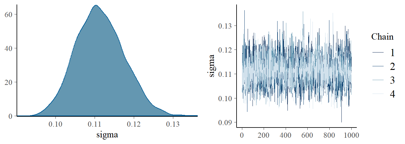
9.6.2 9M2
Modify the terrain ruggedness model again. This time, change the prior for b[cid] to dexp(0.3). What does this do to the posterior distribution? Can you explain it?
今度は、R_cにかかる係数の事前分布をExponential(0.3)にする。これは、事前分布を正に限定していることになる。
b9.1_exp <-
brm(data = d2,
family = gaussian,
formula = bf(G ~ 0 + a + b*R_c,
a ~ 0 + A,
b ~ 0 + A,
nl = TRUE),
prior = c(prior(normal(1, 0.1), class = b, nlpar = a),
prior(exponential(0.3),class=b,nlpar = b),
prior(uniform(0,1), class=sigma)),
seed = 9, chain =4, cores=4,
backend = "cmdstanr",
file = "output/Chapter9/b9.1_exp")かなり警告が出ていて、b_A2の係数が正になってしまっている。他のパラメータの推定はほとんど変わらないが、有効サンプルサイズはかなり少なくなっている。
print(b9.1_exp)## Family: gaussian
## Links: mu = identity; sigma = identity
## Formula: G ~ 0 + a + b * R_c
## a ~ 0 + A
## b ~ 0 + A
## Data: d2 (Number of observations: 170)
## Draws: 4 chains, each with iter = 2000; warmup = 1000; thin = 1;
## total post-warmup draws = 4000
##
## Population-Level Effects:
## Estimate Est.Error l-95% CI u-95% CI Rhat Bulk_ESS Tail_ESS
## a_A1 0.89 0.02 0.86 0.92 1.01 383 618
## a_A2 1.05 0.01 1.03 1.07 1.01 548 891
## b_A1 0.15 0.07 0.02 0.30 1.00 489 972
## b_A2 0.02 0.02 0.00 0.06 1.01 320 701
##
## Family Specific Parameters:
## Estimate Est.Error l-95% CI u-95% CI Rhat Bulk_ESS Tail_ESS
## sigma 0.11 0.01 0.10 0.13 1.00 499 851
##
## Draws were sampled using sample(hmc). For each parameter, Bulk_ESS
## and Tail_ESS are effective sample size measures, and Rhat is the potential
## scale reduction factor on split chains (at convergence, Rhat = 1).posterior_summary(b9.1_exp) %>%
data.frame() %>%
rownames_to_column(var = "parameters") %>%
filter(parameters != "lp__") %>%
gt()| parameters | Estimate | Est.Error | Q2.5 | Q97.5 |
|---|---|---|---|---|
| b_a_A1 | 0.88738587 | 0.016264158 | 0.8550791750 | 0.91906462 |
| b_a_A2 | 1.04853402 | 0.010236978 | 1.0286857500 | 1.06822025 |
| b_b_A1 | 0.14937156 | 0.070870054 | 0.0225516525 | 0.29556600 |
| b_b_A2 | 0.01693269 | 0.015985722 | 0.0005696201 | 0.05762359 |
| sigma | 0.11395191 | 0.006049614 | 0.1030100000 | 0.12689643 |
| lprior | -0.46087953 | 0.189949524 | -0.8744978750 | -0.12167350 |
b_A2のchainだけおかしなことになっている。
##全部
posterior_samples(b9.1_exp, add_chain = TRUE) %>%
dplyr::select(-iter, -lp__) %>%
mcmc_trace(size = .25)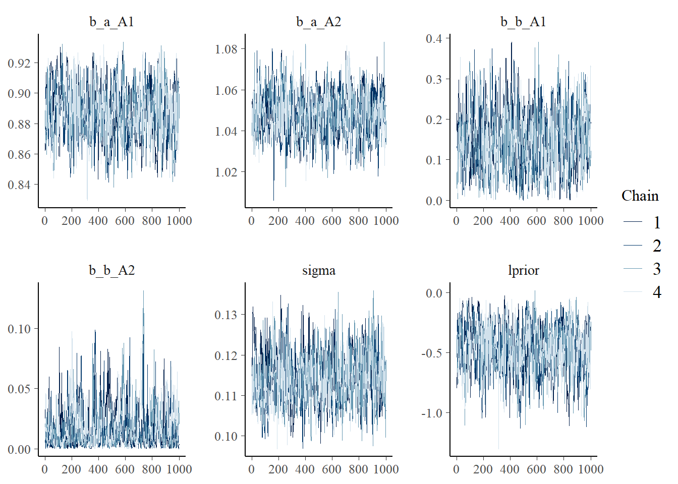
posterior_samples(b9.1_exp, add_chain =TRUE) %>%
dplyr::select(-iter, -lp__) %>%
mcmc_rank_overlay()+
coord_cartesian(ylim = c(30,NA))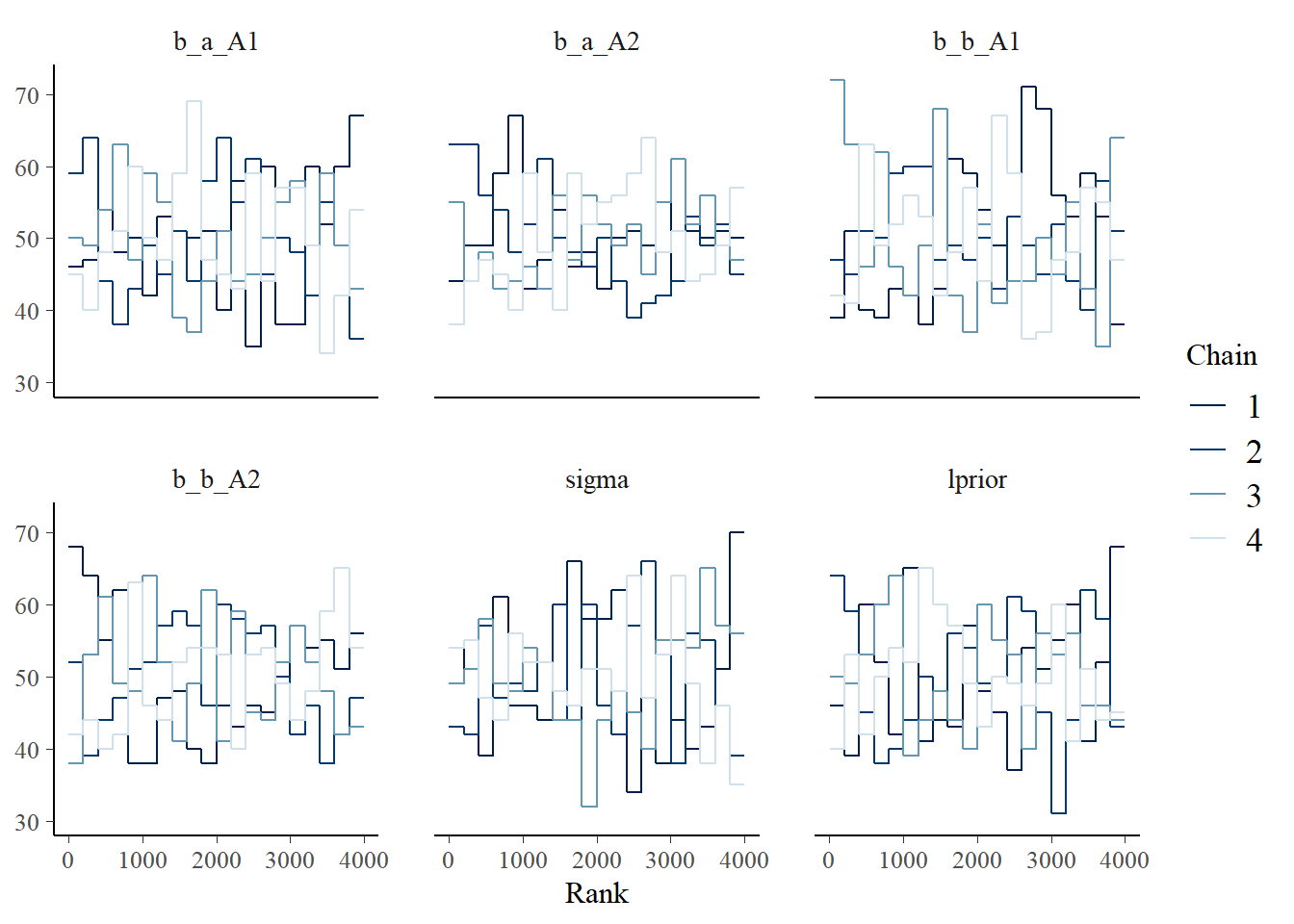
## b_A2のみ
posterior_samples(b9.1_exp, add_chain = TRUE) %>%
mcmc_trace(size = .25,
pars = "b_b_A2")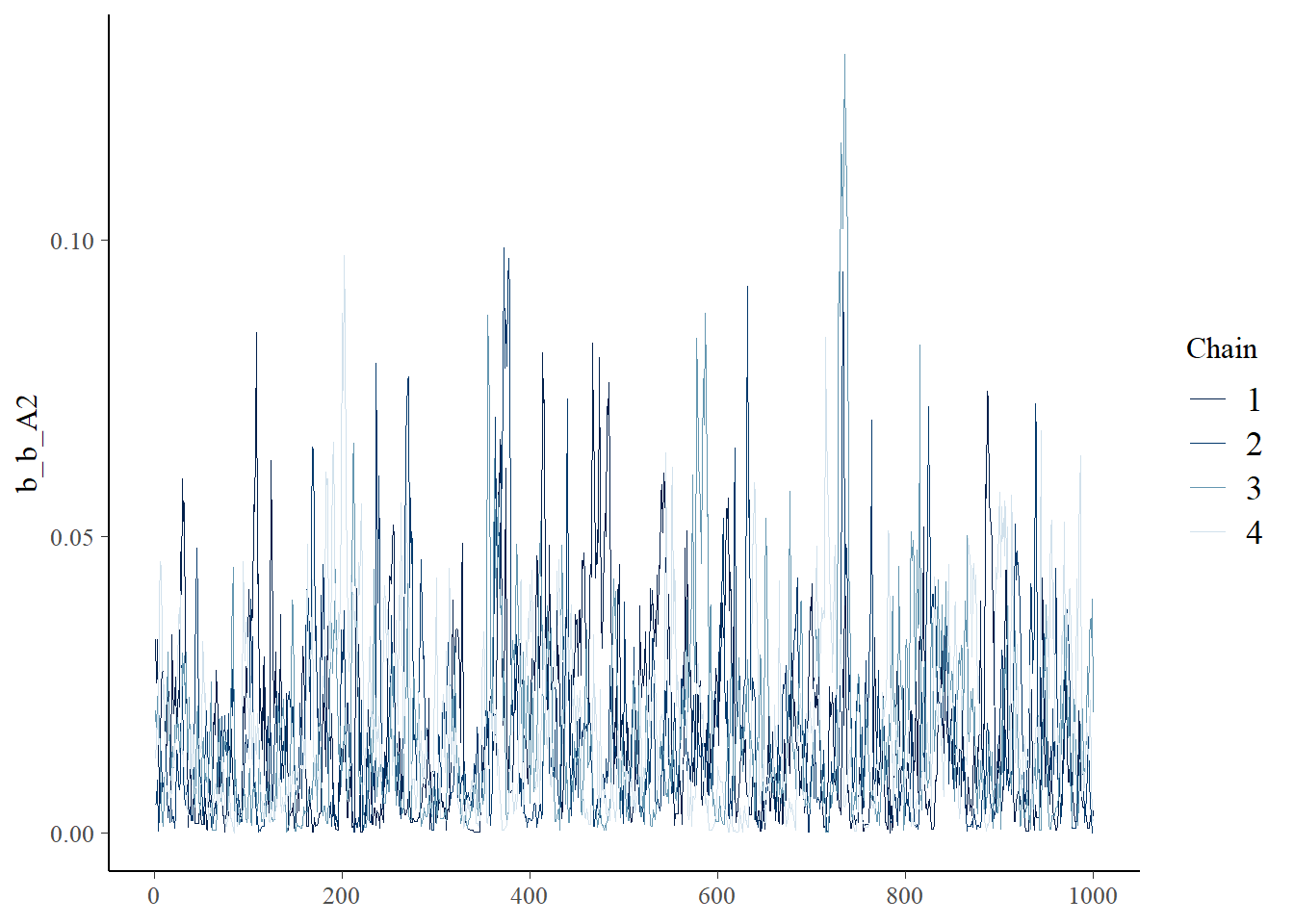
posterior_samples(b9.1_exp, add_chain =TRUE) %>%
mcmc_rank_overlay(pars = "b_b_A2")+
coord_cartesian(ylim = c(30,NA))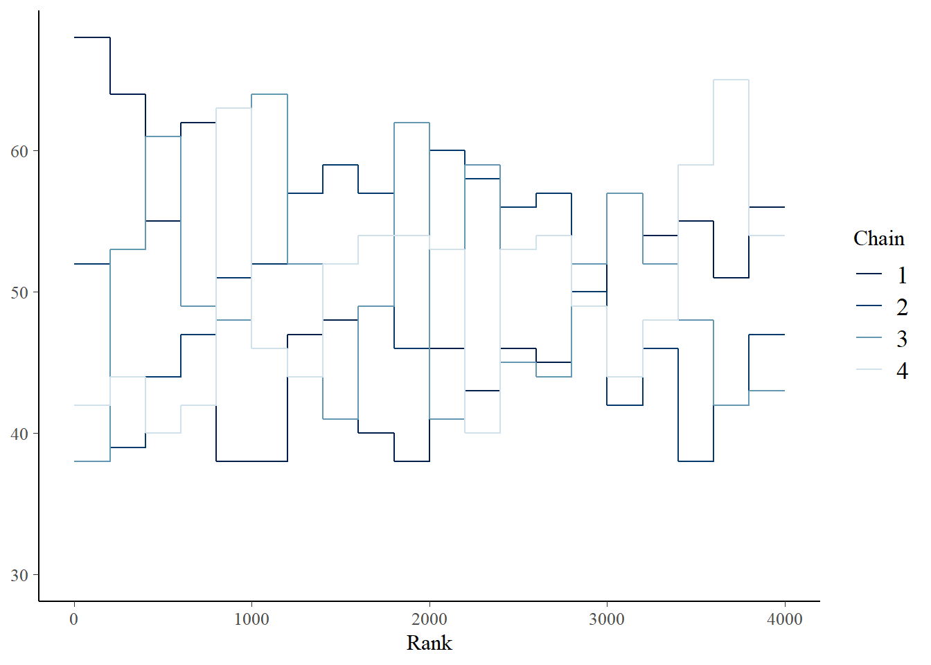
posterior_samples(b9.1_exp, add_chain =TRUE) %>%
mcmc_dens(pars = "b_b_A2")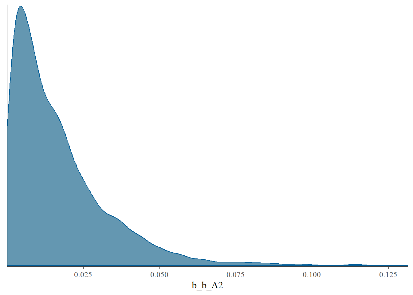
9.6.3 9M3
Re-estimate one of the Stan models from the chapter, but at different numbers of warmup iterations. Be sure to use the same number of sampling iterations in each case. Compare the n_eff values.
b9.1bについてwarmupの回数を変えてみる(5,10,100,500,1000,1500)。
そもそもwarmupが5と10ではdivergence transitionが起きてしまう。それ以後は特に大きな差はない。
list <- list(5,10,100,500,1000,1500)
no_eff <- function(w){
r <- update(b9.1b,
chains = 4, cores=4, iter=1000+w, warmup=w,
seed=9)
}
purrr::map(list, no_eff)## [[1]]
## Family: gaussian
## Links: mu = identity; sigma = identity
## Formula: G ~ 0 + a + b * R_c
## a ~ 0 + A
## b ~ 0 + A
## Data: d2 (Number of observations: 170)
## Draws: 4 chains, each with iter = 1005; warmup = 5; thin = 1;
## total post-warmup draws = 4000
##
## Population-Level Effects:
## Estimate Est.Error l-95% CI u-95% CI Rhat Bulk_ESS Tail_ESS
## a_A1 1.00 0.10 0.91 1.16 17.53 4 NA
## a_A2 1.22 0.20 0.96 1.51 9.45 4 NA
## b_A1 0.72 0.55 0.14 1.61 22.81 4 4
## b_A2 0.72 1.30 -1.51 1.63 26.63 4 4
##
## Family Specific Parameters:
## Estimate Est.Error l-95% CI u-95% CI Rhat Bulk_ESS Tail_ESS
## sigma 0.35 0.11 0.23 0.52 10.12 4 4
##
## Draws were sampled using sampling(NUTS). For each parameter, Bulk_ESS
## and Tail_ESS are effective sample size measures, and Rhat is the potential
## scale reduction factor on split chains (at convergence, Rhat = 1).
##
## [[2]]
## Family: gaussian
## Links: mu = identity; sigma = identity
## Formula: G ~ 0 + a + b * R_c
## a ~ 0 + A
## b ~ 0 + A
## Data: d2 (Number of observations: 170)
## Draws: 4 chains, each with iter = 1010; warmup = 10; thin = 1;
## total post-warmup draws = 4000
##
## Population-Level Effects:
## Estimate Est.Error l-95% CI u-95% CI Rhat Bulk_ESS Tail_ESS
## a_A1 0.89 0.02 0.86 0.92 1.08 118 112
## a_A2 1.05 0.01 1.03 1.07 1.33 18 6
## b_A1 0.13 0.13 -0.07 0.38 1.62 7 12
## b_A2 -0.12 0.12 -0.26 0.08 1.31 10 52
##
## Family Specific Parameters:
## Estimate Est.Error l-95% CI u-95% CI Rhat Bulk_ESS Tail_ESS
## sigma 0.12 0.01 0.10 0.15 1.40 9 29
##
## Draws were sampled using sampling(NUTS). For each parameter, Bulk_ESS
## and Tail_ESS are effective sample size measures, and Rhat is the potential
## scale reduction factor on split chains (at convergence, Rhat = 1).
##
## [[3]]
## Family: gaussian
## Links: mu = identity; sigma = identity
## Formula: G ~ 0 + a + b * R_c
## a ~ 0 + A
## b ~ 0 + A
## Data: d2 (Number of observations: 170)
## Draws: 4 chains, each with iter = 1100; warmup = 100; thin = 1;
## total post-warmup draws = 4000
##
## Population-Level Effects:
## Estimate Est.Error l-95% CI u-95% CI Rhat Bulk_ESS Tail_ESS
## a_A1 0.89 0.02 0.86 0.92 1.00 4260 3024
## a_A2 1.05 0.01 1.03 1.07 1.00 4568 2992
## b_A1 0.13 0.07 -0.01 0.28 1.00 1667 1697
## b_A2 -0.14 0.06 -0.25 -0.03 1.00 2618 1956
##
## Family Specific Parameters:
## Estimate Est.Error l-95% CI u-95% CI Rhat Bulk_ESS Tail_ESS
## sigma 0.11 0.01 0.10 0.12 1.00 2316 2070
##
## Draws were sampled using sampling(NUTS). For each parameter, Bulk_ESS
## and Tail_ESS are effective sample size measures, and Rhat is the potential
## scale reduction factor on split chains (at convergence, Rhat = 1).
##
## [[4]]
## Family: gaussian
## Links: mu = identity; sigma = identity
## Formula: G ~ 0 + a + b * R_c
## a ~ 0 + A
## b ~ 0 + A
## Data: d2 (Number of observations: 170)
## Draws: 4 chains, each with iter = 1500; warmup = 500; thin = 1;
## total post-warmup draws = 4000
##
## Population-Level Effects:
## Estimate Est.Error l-95% CI u-95% CI Rhat Bulk_ESS Tail_ESS
## a_A1 0.89 0.02 0.86 0.92 1.00 4816 3212
## a_A2 1.05 0.01 1.03 1.07 1.00 4834 3104
## b_A1 0.13 0.07 -0.01 0.28 1.00 4546 3021
## b_A2 -0.14 0.05 -0.25 -0.04 1.00 4508 2896
##
## Family Specific Parameters:
## Estimate Est.Error l-95% CI u-95% CI Rhat Bulk_ESS Tail_ESS
## sigma 0.11 0.01 0.10 0.12 1.00 4789 3463
##
## Draws were sampled using sampling(NUTS). For each parameter, Bulk_ESS
## and Tail_ESS are effective sample size measures, and Rhat is the potential
## scale reduction factor on split chains (at convergence, Rhat = 1).
##
## [[5]]
##  Family: gaussian
##   Links: mu = identity; sigma = identity
## Formula: G ~ 0 + a + b * R_c
##          a ~ 0 + A
##          b ~ 0 + A
##    Data: d2 (Number of observations: 170)
##   Draws: 4 chains, each with iter = 2000; warmup = 1000; thin = 1;
##          total post-warmup draws = 4000
##
## Population-Level Effects:
##      Estimate Est.Error l-95% CI u-95% CI Rhat Bulk_ESS Tail_ESS
## a_A1     0.89      0.02     0.86     0.92 1.00     4788     3163
## a_A2     1.05      0.01     1.03     1.07 1.00     4423     3086
## b_A1     0.13      0.07    -0.02     0.28 1.00     4279     2983
## b_A2    -0.14      0.06    -0.25    -0.03 1.00     4892     2828
##
## Family Specific Parameters:
##       Estimate Est.Error l-95% CI u-95% CI Rhat Bulk_ESS Tail_ESS
## sigma     0.11      0.01     0.10     0.12 1.00     4850     2996
##
## Draws were sampled using sampling(NUTS). For each parameter, Bulk_ESS
## and Tail_ESS are effective sample size measures, and Rhat is the potential
## scale reduction factor on split chains (at convergence, Rhat = 1).
##
## [[6]]
## Family: gaussian
## Links: mu = identity; sigma = identity
## Formula: G ~ 0 + a + b * R_c
## a ~ 0 + A
## b ~ 0 + A
## Data: d2 (Number of observations: 170)
## Draws: 4 chains, each with iter = 2500; warmup = 1500; thin = 1;
## total post-warmup draws = 4000
##
## Population-Level Effects:
## Estimate Est.Error l-95% CI u-95% CI Rhat Bulk_ESS Tail_ESS
## a_A1 0.89 0.02 0.86 0.92 1.00 5188 2933
## a_A2 1.05 0.01 1.03 1.07 1.00 4582 3237
## b_A1 0.13 0.08 -0.02 0.28 1.00 4577 3089
## b_A2 -0.14 0.06 -0.25 -0.03 1.00 4871 3113
##
## Family Specific Parameters:
## Estimate Est.Error l-95% CI u-95% CI Rhat Bulk_ESS Tail_ESS
## sigma 0.11 0.01 0.10 0.12 1.00 4782 3087
##
## Draws were sampled using sampling(NUTS). For each parameter, Bulk_ESS
## and Tail_ESS are effective sample size measures, and Rhat is the potential
## scale reduction factor on split chains (at convergence, Rhat = 1).9.6.4 9H1
Run the model below and then inspect the posterior distribution and explain what it is accomplishing.
単に事前分布からサンプリングしていることになる。
bのtraceplotがところどころ極端な値に飛んでいるのは、コーシー分布が非常に幅広い裾を持つからである。この場合、bのtraceplotは問題ない。
mp <- brm(bf(1 ~ a + b, a ~ 1, b ~ 1, nl = TRUE), data = 1,
          prior = c(prior(normal(0, 1), class = b, nlpar = a),
                    prior(cauchy(0, 1), class = b, nlpar = b)),
          iter = 2000, chains = 1, sample_prior = "only",
          file = "output/Chapter9/mp")

as_draws_df(mp, variable = "^b_", regex = TRUE) %>%
  as_tibble() %>%
  pivot_longer(starts_with("b_"), names_to = "param") %>%
  mutate(param = str_replace_all(param, "b_([ab])_Intercept", "\\1")) %>%
  ggplot(aes(x = .draw, y = value)) +
  facet_wrap(~param, nrow = 1, scales = "free_y") +
  geom_line(color = "#009FB7")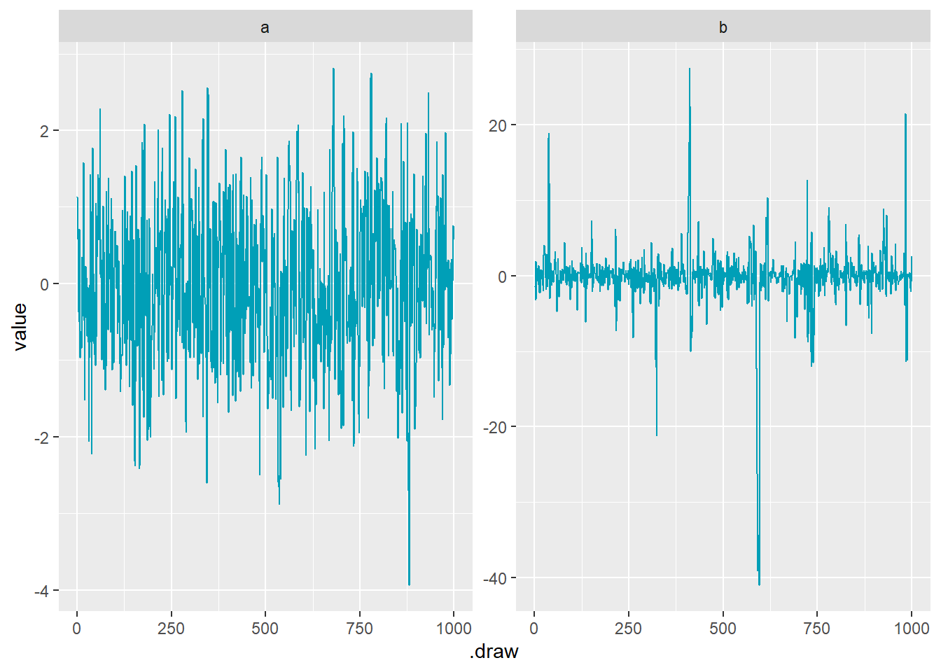
9.6.5 9H2
Recall the divorce rate example from Chapter 5. Repeat that analysis, using ulam() this time, fitting models m5.1, m5.2, and m5.3. Use compare to compare the models on the basis of WAIC or PSIS. Explain the results.
b5.1 <- readRDS("output/Chapter5/b5.1.rds")
b5.2 <- readRDS("output/Chapter5/b5.2.rds")
b5.3 <- readRDS("output/Chapter5/b5.3.rds")

loo_compare(b5.1,b5.2,b5.3) %>%
  print(simplify = FALSE)
## elpd_diff se_diff elpd_loo se_elpd_loo p_loo se_p_loo looic se_looic
## b5.1 0.0 0.0 -62.9 6.4 3.7 1.8 125.9 12.8
## b5.3 -0.9 0.4 -63.8 6.4 4.8 1.9 127.7 12.9
## b5.2 -6.7 4.6 -69.6 4.9 2.9 0.9 139.2 9.89.6.6 9H3
Sometimes changing a prior for one parameter has unanticipated effects on other parameters. This is because when a parameter is highly correlated with another parameter in the posterior, the prior influences both parameters. Here’s an example to work and think through. Go back to the leg length example in Chapter 5. Here is the code again, which simulates height and leg lengths for 100 imagined individuals:
set.seed(909)
n <- 100

d <- tibble(height = rnorm(n, 10, 2),
            leg_prop = runif(n, 0.4, 0.5)) %>%
     mutate(leg_left = leg_prop*height +
              rnorm(n,0,0.02),
            leg_right = leg_prop*height +
              rnorm(n, 0, 0.02))
b9H3 <-
brm(data = d,
family = gaussian,
formula = height ~ 1 + leg_left + leg_right,
prior = c(prior(normal(10,100),class=Intercept),
prior(normal(2,10),class=b),
prior(exponential(1),class = sigma)),
iter=2000,warmup=1000,chains=4,
backend = "cmdstanr",
file = "output/Chapter9/b9H3")
b9H3_2 <-
brm(data = d,
family = gaussian,
formula = bf(height ~ a + b + c,
a ~ 0 + leg_left,
b ~ 0 + leg_right,
c ~ 1,
nl = TRUE),
prior = c(prior(normal(10,100),nlpar = c),
prior(normal(2,10),nlpar = a),
prior(normal(2,10),nlpar =b,lb =0),
prior(exponential(1),class = sigma)),
iter=2000,warmup=1000,chains=4,
backend = "cmdstanr",
file = "output/Chapter9/b9H3_2")もともとの制約なしのモデル。
pairs(b9H3,
      off_diag_args = list(size = 1/5, alpha = 1/5))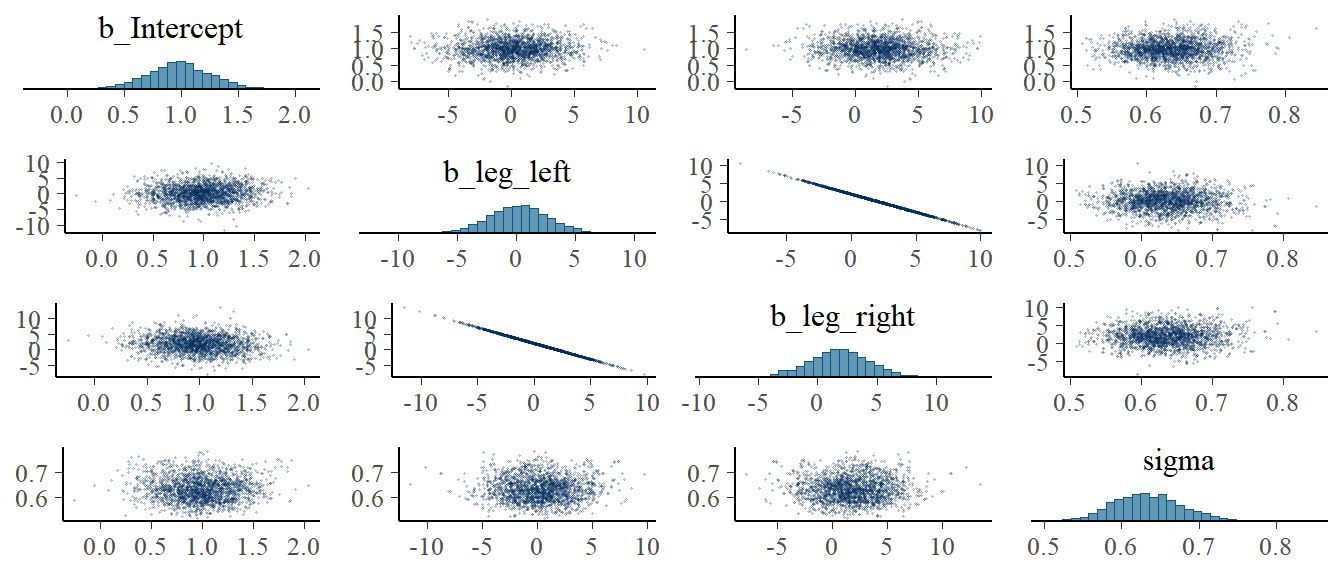
右脚の係数の事前分布を正に制約したモデル。
右脚と左脚は強く相関していたので、右脚の係数が左に傾いたことで左脚の係数が右に傾いた。
pairs(b9H3_2,
      off_diag_args = list(size = 1/5, alpha = 1/5))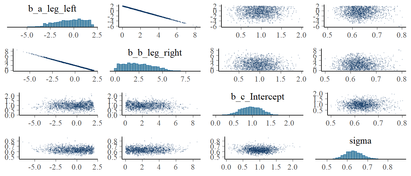
9.6.7 9H4
For the two models fit in the previous problem, use WAIC or PSIS to compare the effective numbers of parameters for each model. You will need to use log_lik=TRUE to instruct ulam() to compute the terms that both WAIC and PSIS need. Which model has more effective parameters? Why?
2つめのモデルの方がPSISが小さい。これは、事前分布が制約されたことによって、事後分布の分散が小さくなったからだと考えられる。
b9H3 <- add_criterion(b9H3, c("loo","waic"))
b9H3_2 <- add_criterion(b9H3_2, c("loo","waic"))

loo_compare(b9H3, b9H3_2) %>%
  print(simplify=FALSE)
## elpd_diff se_diff elpd_loo se_elpd_loo p_loo se_p_loo looic se_looic
## b9H3_2 0.0 0.0 -97.1 5.7 2.7 0.4 194.1 11.3
## b9H3 -0.5 0.2 -97.6 5.6 3.2 0.5 195.1 11.29.6.8 9H5
Modify the Metropolis algorithm code from the chapter to handle the case that the island populations have a different distribution than the island labels. This means the island’s number will not be the same as its population.
set.seed(9)

num_weeks <- 1e6
positions <- rep(0, num_weeks)
current <- 10

## 各島の人口をランダムに決定する
population <- sample(1:10)

## アルゴリズムの記述
for(i in 1:num_weeks){
  positions[i] <- current
  proposal <- current + sample(c(-1,1), size=1)

  if(proposal <1)  proposal <- 10
  if(proposal >10) proposal <- 1

  prob_move <- population[proposal]/population[current]
  current <- ifelse(runif(1) < prob_move, proposal, current)
}
人口をランダムに振り分けてもうまく働くことが分かった。
tibble(week = 1:1e6,
       island = positions) %>%
  count(island) %>%
  mutate(population = population) %>%
  mutate(prop = n/n[population=="1"]) %>%
  gt() %>%
  fmt_number("prop",decimals=2) %>%
tab_options(table.align='left')| island | n | population | prop |
|---|---|---|---|
| 1 | 91653 | 5 | 5.06 |
| 2 | 109872 | 6 | 6.06 |
| 3 | 54369 | 3 | 3.00 |
| 4 | 144904 | 8 | 7.99 |
| 5 | 126778 | 7 | 6.99 |
| 6 | 72408 | 4 | 3.99 |
| 7 | 181812 | 10 | 10.03 |
| 8 | 163674 | 9 | 9.03 |
| 9 | 36400 | 2 | 2.01 |
| 10 | 18130 | 1 | 1.00 |
9.6.9 9H6
Modify the Metropolis algorithm code from the chapter to write your own simple MCMC estimator for globe tossing data and model from Chapter 2.
コインは{W,L,W,W,W,L,W,L,W}の順番で落ちた。
## 以下アルゴリズム
w <- 6
n <- 9
iter=1e4

p_prior <- function(p) dunif(p, min=0,max=1)
p_sample <- rep(0, iter)
p_current <- 0.5

for(i in 1:iter){
  p_sample[i] <- p_current
  p_proposal <- runif(1,min=0,max=1)
  prob_current <- dbinom(w,n,p_current)*p_prior(p_current)
  prob_proposal <- dbinom(w,n,p_proposal)*p_prior(p_proposal)

  prob_move <- prob_proposal/prob_current
  p_current <-ifelse(runif(1) < prob_move,
                     p_proposal, p_current)
}
上手く推定できていそう。
tibble(iter = 1:iter,
       prob = p_sample) %>%
  ggplot(aes(x=iter, y = prob))+
  geom_line()+
  theme_bw()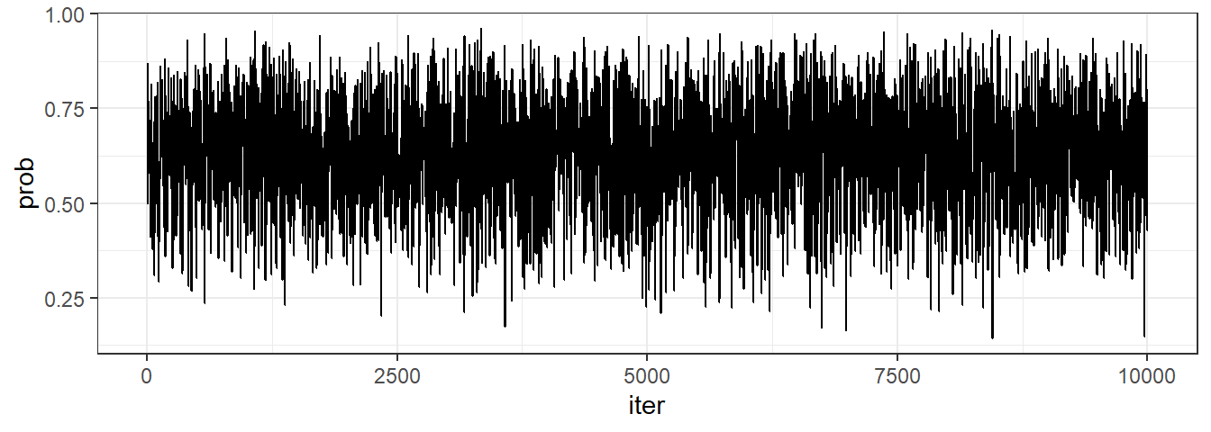
tibble(iter = 1:iter,
       prob = p_sample) %>%
  ggplot(aes(x=prob))+
  geom_histogram(binwidth = 0.1)+
  stat_function(fun=function(x) iter*dbinom(w,n,x),
                color = "red")+
  labs(y = "Density")+
  theme_bw()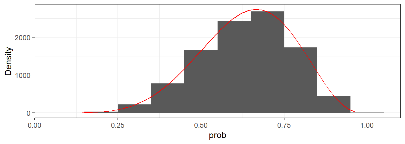
mean_qi(p_sample) %>%
gt()| y | ymin | ymax | .width | .point | .interval |
|---|---|---|---|---|---|
| 0.6354329 | 0.3450299 | 0.8791578 | 0.95 | mean | qi |